Input Data

Belgian energy system data in 2035

Overview This appendix reports the input data for the application of the LP modeling framework to the case study of Belgium between 2015 and 2050. Data are detailed for the year 2035 and 2015, the latter used for model verification. Trends to extrapolated these data for the other years are given. This appendix is an improved version previously presented in ^2,6

The data can be grouped into three parts: resources (Section Resources), demand (Section Demand) and technologies (Section Technologies.. For resources, the work of the JRC ³⁷, Biomass atlas ³⁸ and Hydrogen Import Coalition³⁹ have been used to complement and confirm or correct the prices already reported in previous works ^2,5,11. For energy demand, the annual demand is calculated from the work of the European Commission’s projections up to 2050 ²⁷. As a complement, the time series are all calculated on the basis of the year 2015. For technologies, they are characterised by the following characteristics: energy balances, cost (investment and maintenance), and environmental impact (global warming potential (GWP)). For weather dependent technologies (wind, solar, etc.), real production for the year 2015 was collected from the TSO.

For GWP and GHG emissions, LCA data are taken from the Ecoinvent database v3.2 [1] ⁴⁰ using the “allocation at the point of substitution” method. GWP is assessed with the “GWP100a - IPCC2013” indicator. For technologies, the GWP impact accounts for the technology construction; for resources, it accounts for extraction, transportation and combustion. In addition, data for fuel combustion are taken from Quaschning⁴¹.

For the cost, the reported data are the nominal values for Belgium in the year 2035 All costs are expressed in real [2] Euros for the year 2015 (€₂₀₁₅). If not specified, € refers to €₂₀₁₅. All cost data used in the model originally expressed in other currencies or referring to another year are converted to €₂₀₁₅ to offer a coherent comparison. Most of the data come from a previous work ^2,5, and were expressed in CHF₂₀₁₅ (Based on the average annual exchange rate value from ECB https://www.ecb.europa.eu, the annual rate was 1€₂₀₁₅ = 1.0679CHF₂₀₁₅). The method used for the year conversion is illustrated by Eq. (43).

(43)\[c_{inv} [\text{€}_{2015}] = c_{inv} [C_y] \cdot \frac{\text{USD}_y}{C_y} \cdot \frac{\text{CEPCI}_{2015} \ [\text{USD}_{2015}]}{\text{CEPCI}_y \ [\text{USD}_y]} \cdot \frac{\text{€}_{2015}}{\text{USD}_{2015}}\]

Where \(C\) and \(y\) are the currency and the year in which the original cost data are expressed, respectively, USD is the symbol of American Dollars and the CEPCI ⁴² is an index taking into account the evolution of the equipment cost (values reported in Table 5). As an example, if the cost data are originally in EUR₂₀₁₀, they are first converted to USD₂₀₁₀, then brought to USD₂₀₁₅ taking into account the evolution of the equipment cost (by using the CEPCI), and finally converted to €₂₀₁₅. The intermediate conversion to USD is motivated by the fact that the CEPCI is expressed in nominal USD. Although this conversion method is originally defined for technology-related costs, in this paper as a simplification it used also for the cost of resources.

Table 5 CEPCI values ⁴²

Year	CEPCI
1982	285.8
1990	357.6
1991	362.3
1992	367.0
1993	371.7
1994	376.4
1995	381.1
1996	381.7
1997	386.5
1998	389.5
1999	390.6
2000	394.1
2001	394.3
2002	395.6
2003	402.0
2004	444.2
2005	468.2
2006	499.6
2007	525.4
2008	575.4
2009	521.9
2010	550.8
2011	585.7
2012	584.6
2013	567.3
2014	576.1
2015	556.3

Resources

Resources can be regrouped in two categories: endogenous and exogenous. In the case of Belgium, endogenous resources are exclusively renewables. They account for solar, biomass, wind and hydro. The only endogenous resource which is non renewable is waste. In addition, energy can be imported from abroad (exogenous). These resources are characterised by an import price and a maximum potential. Exogenous resources account for the import of hydrocarbons, electricity or other fuels.

The availability of all resources, except for biomass, and non-RE waste, is set to a value high enough to allow unlimited use in the model. Table 8 details the prices of resources (\(c_{op}\)), the GHG emissions (\(gwp_{op}\)) associated to their production, transportation and combustion; and endogenous availability of resources. Export of electricity are possible, but they are associated to a zero selling price. Two kinds of emissions are proposed: one accounting for the impact associated to production, transport and combustion (based on GWP100a - IPCC2013 ⁵); the other accounting only for combustion (based on Quaschning⁴¹). Total emissions are used to assess energy system emissions. Combustion only is used to calculate the direct CO2 emissions that can be captured and used through a carbon capture technology (latter presented).

Local renewable resources

The majors renewable potentials are: solar, biomass and wind. Additionnaly, Belgium has hydro and perhaps affordable geothermal. Wind, solar, hydro and geothermal are limited by the number of technologies deployable, while biomass is limited by the amount of resources available.

Wind, solar, hydro and geothermal

The energy transition relies on renewable energies, which makes their deployment potential a critical parameter. In 2015, 6% of the primary energy consumed in Belgium was renewable, mainly biomass, solar and wind. In the following, we summarise the potential for the different resources: in terms of available potential for biomass and waste (Table 6); or in terms of capacity for solar, wind, geothermal and hydro (Table 7). These data are put into perspective with the real data for 2015.

Table 6 Comparison of installed capacity of renewable energies (RE) based technologies in 2015 and their potentials in the model. Abbreviations: centralised (cen.), decentralised (dec.), maximum (max.).

Technology	2015 [aa]	max. potential	Units
photovoltaic	3.85	\(\approx\)60 [bb]	[GW]
onshore wind	1.18	10 [cc]	[GW]
offshore wind	0.69	3.5	[GW]
hydro river	0.11 [dd]	0.120	[GW]
geothermal	0	\(\approx\)0 [ee]	[GW]
geothermal	\(\approx\)0	\(\approx\)0	[GW]
cen. solar th.	0	\(\approx\) 70	[GW]
dec. solar th.	0	\(\approx\) 70	[GW]

[aa]

Data from ⁶ consistent with Eurostat ⁴³.

[bb]

Due to land availability, the solar potentials are limited to around 1% of total Belgian lands (250km\(^2\)). This is equivalent to \(\approx\)60 GW of PV or \(\approx\)70 GW of solar thermal.

[cc]

From ⁴⁴. In line with ⁴⁵ which estimated 9 GW for onshore and 8 GW for offshore.

[dd]

In 2015, the production was 360 GWh ²⁷ with an installed capacity of around 110 MW ⁴⁶. No important development is foreseen ^45,46.

[ee]

A prototype (Balmatt project) started in 2019 and should produce 4-5 MW ⁴⁷.

Table 7 Renewable resources in 2015 and their potential.

Resources	2015	max. potential	Units
bioethanol	0.48 [ff]	0	[TWh]
biodiesel	2.89	0	[TWh]
SNG	0	0	[TWh]
H2	0	0	[TWh]
woody [gg]	13.9	23.4	[TWh]
wet	11.6 [hh]	38.9	[TWh]
7.87	17.8	[TWh]

[ff]

Bioethanol also accounts for other bio-fuels except biodiesel. In 2015, 0.21 TWh of bioethanol have been imported, the rest of the biofuels have been produced locally from crops . In the model, the crops available to produce sustainable biomass are accounted for, and can produce wet or woody biomass.

[gg]

Endogenous potential. See following section.

[hh]

Belgium production of bioethanol, biomethanol, biogas and biodiesel is accounted for as wet biomass.

Wind, solar and biomass are foreseen to be the main resources. The land availability for PV is highly speculative, we propose a simple approach to estimate an order of magnitude of this limit. Assuming that it exists today 250 km\(^2\) of available well oriented roof [9] ⁴⁶ and that the efficiency in 2035 will be 23% ³⁵ with an average daily total irradiation - similar to historical values - of 2820 Wh/m\(^2\) in Belgium ³⁶. The upper limit becomes 59.2 GW of installed capacity [10]. This limit is in line with a study performed by the Belgian TSO which proposes arbitrarily 40 GW ⁴⁵. The hydro potential is very limited and almost fully exploited. Even if geothermal heat is used for heating through DHN since 1986 at Saint Ghislain ⁴⁸, research about the geothermal potential in Belgium are at their early stages. In 2015, a new project started (the Balmatt project). Nowadays, the installation produces 1.5 MW of electricity (in 2019). The project is expected to scale up to 5 MW of electricity ⁴⁷. However, there is no large facility yet and the potential is not accurately estimated. A study performed by the VITO evaluates the potential in Flanders to 3.1 GWe and they extend it to 4 GWe for the whole Belgian potential ⁴⁶. However, because of a lack of reliable sources about geothermal potential, we consider the potential as null in the reference scenario.

The wind potential is estimated to 10 GW onshore and 3.5 GW offshore ⁴⁴. At the time of collecting the data (2011-2020), several potentials can be collected through various sources. As an example, the study from Devogelaer et al.⁴⁶ proposes to use 9 GW and 8 GW for onshore and offshore, respectively. As another example, Dupont et al.⁴⁹ estimates the wind potential based on its energy return on invested energy, in other words, its profitability. This study concluded that Belgium has a potential between 7 660 and 24 500 MW for onshore and between 613 and 774 MW for offshore [11]. At the time of writing, the wind energy is in the spotlight with collapsing investment costs and a rising potential. Indeed, Europe has one of the best potential worldwide and has a leading wind power industry. As an illustration of recent improvements the following argument motivates the increase of the Belgian wind potential: taller and taller wind turbines enable the use of faster and more constant wind. As a consequence, the offshore potential might be underestimated. On the other hand, the onshore potential might be overestimated as developers see their project often blocked by citizens. In a nutshell, the wind potential allowed is relevant, but perhaps slightly underestimated. As motivated in the results, due to its limited potential, wind will remain a small contributor of the energy mix with a maximum of \(\approx\)10%.

Biomass and non-RE waste

In the literature, waste and biomass are often merged, as it is the case in the European commission report ²⁷. In this thesis, a distinction is made between biomass and waste. Waste accounts for all the fossil waste, such as plastics, whereas biomass is organic and assumed renewable. Biomass is split into two categories: one that can be digested by bacteria (wet biomass), such as apple peel; and one that cannot (woody biomass), such as wood. Hence, the organic waste generated by the municipalities is accounted for in woody or wet biomass and not as fossil waste.

In the literature, biomass potential highly varies based on the assumptions made, such as the area available to produce biomass, or the definition of sustainable biomass. In an European study, Elbersen et al.³⁸ drew the biomass atlas of EU countries for different scenarios in terms of prices and potentials. According to a conservative approach, the sustainable scenario estimations are selected. In their work, biomass is declined in a larger variety of form. To adapt these data to our work, these varieties are aggregated into three types: woody biomass, wet biomass and non-RE waste. Waste accounts for common sludges, MSW landfill, MSW not landfill (composting, recycling) and paper cardboard. The overall potential is estimated to 17.8 TWh/y with an approximate price of 10.0 €/MWh. The price is estimated as a weighted sum between the different variety and their specific price (given in the document). Wet biomass accounts for all the digestible biomass, which are verge gras, perennials (grassy), prunings, total manure, grass cuttings abandoned grassland, animal waste and forrage maize (biogas). The overall potential is estimated to 38.9 TWh/y with an approximate price of 2.5 €/MWh. Woody biomass accounts for all the non-digestible biomass, which are roundwood (including additional harvestable roundwood), black liquor, landscape care wood, other industrial wood residues, perennials (woody), post consumer wood, saw-dust, sawmill by-products (excluding sawdust) and primary forestry residues. The overall potential is estimated to 23.4 TWh/y with an approximate price of 14.3 €/MWh.

Oleaginous (0.395 TWh/y) and sugary (0 TWh/y) potentials are two order of magnitude below the previous categories and thus neglected.

However, these costs do not account for treatment and transportation. Based on a local expert (from Coopeos), a MWh of wood ready to use for small wood boilers is negotiated around 28 €/MWh today, twice much than estimated prices. This order of magnitude is in line with the Joint Research Center price estimation in 2030 ³⁷. Thus, the price proposed in ³⁸ are doubled. It results in prices for woody biomass, wet biomass and waste of 28.5, 5.0 and 20.0 €/MWh in 2015, respectively. The price for biomass is expected to increase by 27.7% up to 2050 ³⁷. By adapting these value to 2035, the prices are for 32.8 €/MWh woody biomass, 5.8 €/MWh for wet biomass and for 23.1 €/MWh for waste.

Imported resources

Dominating fossil fuels are implemented in the model and detailed in Section [ssec:case_study_imported_res]. They can be regrouped in hydrocabons (gasoline, diesel, LFO and NG), coal and uranium. Data is summarised in Table 8 and are compared to other sources, such as estimations from the JRC of prices for oil, gas and coal ³⁷. They base their work on a communication of the European Commission ⁵⁰.

There are a long list of candidate to become renewable fuels. Historically, biomass has been converted into bio-fuels. Two types of these fuels are accounted: bio-diesel and bio-ethanol. They can substitute diesel and gasoline, respectively. More recently, a new type of renewable fuel is proposed and can be labeled electro-fuels. Indeed, these fuels are produced from electricity. We consider that the energy content of these fuels is renewable (i.e. from renewable electricity). Four type of fuels were considered: hydrogen, ammonia, methanol and methane. To avoid ambiguity between renewable fuels and their fossil equivalent, it is specified if the imported resources is renewable or fossil.

Caution

to be updated + explain where data comes from.

The only difference being Thus, we have gas and gas_re, or h2 and h2_re. Gas refers to what is usually called ‘natural gas’, while gas_re refers to methane from biogas, methanation of renewable hydrogen,… Since, a specific study for the Belgian case has been conducted by a consortium of industries, Hydrogen Import Coalition³⁹, which estimate new prices for the imports. Table 8 summarises all the input data for the resources.

Table 8 Price, GHG emissions and availability of resources, in 2035. Abbreviations: Liquid Fuel Oil (LFO), Natural Gas (NG) and Synthetic Natural Gas (SNG).

Resources	\(c_ {op}\)	\(gwp_ {op}\)	\({CO}_ {2direct}\) [26]	avail
	[€2015/MWhfuel]	[kgCO2-eq. /MWhfuel]	[kgCO:sub:2/MWhfuel]	[GWh]
Electricity Import	84.3 [27]	206.4 [28]	0	27.5
Gasoline	82.4 [29]	345 [28]	250	infinity
Diesel	79.7 [30]	315 [28]	270	infinity
LFO	60.1 [31]	311.5 [28]	260	infinity
Fossil Gas	44.3 [32]	267 [28]	200	infinity
Woody biomass	32.8	11.8 [28]	390	23.4
Wet-biomass	5.8	11.8 [28]	390	38.9
non-RE waste	23.1	150 [28]	260 [33]	17.8
Coal	17.6	401 40	360	33.3 [37]
Uranium	3.9 [34]	3.9 40	0	infinity
Bio-diesel	120.0	0 [36]_	270	infinity
Bio-gasoline	111.3 [35]	0 [36]_	250	infinity
Renew. gas	118.3	0 [36]_	200	infinity
Fossil H2 [25]	87.5	364	0	infinity
Renew. H2	119.4	0 [36]_	0	infinity
Fossil Ammonia [25]	76	285	0	infinity
Renew. Ammonia	81.8	0 [36]_	0	infinity
Fossil Methanol [25]	82.0	350	246	infinity
Renew. Methanol	111.3	0 [36]_	246	infinity

[25] (1,2,3)

Own calculation for fossil hydrogen, ammonia and methanol. Price and emissions are calculated based on fossil gas and based on conversion efficiencies.

[26]

Direct emissions related to combustion:cite:Quaschning2015.

[27]

Based on average market price in the year 2010 (50 EUR₂₀₁₀/MWh, from ⁵¹). Projected from 2010 to 2035 using a multiplication factor of 1.36 ⁵². For security of supply reason, the availability is limited to 30% of yearly electricity EUD (See Section [ssec:be_policies]).

[28] (1,2,3,4,5,6,7,8)

GWP100a-IPCC2013 metric: impact associated to production, transport and combustion, see ⁵

[29]

Based on 1.49 CHF₂₀₁₅/L (average price in 2015 for gasoline 95 in Switzerland) ⁵³. Taxes (0.86 CHF₂₀₁₅/L, ⁵⁴) are removed and the difference is projected from 2015 to 2035 using a multiplication factor of 1.24 ⁵⁵. In line with ³⁷.

[30]

Based on 1.55 CHF₂₀₁₅/L (average price in 2015) ⁵³. Taxes (0.87 CHF₂₀₁₅/L, ⁵⁴) are removed and the difference is projected from 2015 to 2035 using a multiplication factor of 1.24 ⁵⁵. In line with ³⁷.

[31]

Based on 0.705 CHF₂₀₁₅/L (average price in 2015 for consumptions above 20000 L/y) ⁵⁶. Taxes (0.22 CHF₂₀₁₅/L, ⁵⁴) are removed and the difference is projected from 2015 to 2035 using a multiplication factor of 1.24 ⁵⁵. In line with ³⁷.

[32]

Based on the EUC estimated cost of resources in 2030, see Table 5 from ³⁷.

[33]

Assuming that the energy content can be assimilated to plastics and extended to LFO.

[34]

Average of the data points for 2035 in ⁵⁷, accounting for the efficiency of nuclear power plants (Table 12).

[35]

Data extrapolated from ⁵⁸

[36]

Emissions related to electro-fuels and bio-fuels production are neglected.

[36]

Belgium is phasing out coal. Coal is still used in industrial processes. In 2015, 33.3 TWh of coal were used. Thus, the amount available should be lower than this value.

Energy demand and political framework

The EUD for heating, electricity and mobility in 2035 is calculated from the forecast done by the EUC in 2035 for Belgium (see Appendix 2 in ²⁷). However, in ²⁷, the FEC is given for heating and electricity. The difference between FEC and EUD is detailed in Section [ssec:conceptual_modelling_framework] and can be summarised as follows: the FEC is the amount of input energy needed to satisfy the EUD in energy services. Except for HP, the FEC is greater than EUD. We applied a conservative approach by assuming that the EUD equal to the FEC for electricity and heating demand.

Electricity

The values in table 1.3 list the electricity demand that is not related to heating for the three sectors in 2035. The overall electricity EUD is given in ²⁷. However, only the FEC is given by sectors. In order to compute the share of electricity by sector, we assume that the electricity to heat ratio for the residential and services remain constant between 2015 and 2035. This ratio can be calculated from European Commission - Eurostat.⁵⁹, these ratio of electricity consumed are 24.9% and 58.2% for residential and services, respectively. As a consequence, the industrial electricity demand is equal to the difference between the overall electricity demand and the two other sectors.

A part of the electricity is assumed to be a fixed demand, such as fridges in households and services, or industrial processes. The other part is varying, such as the lighting demand. The ratio between varying electricity and fixed demand are calculated in order to fit the real curve in 2015 (data provided by ENTSO-E https://www.entsoe.eu/). It results in a share of 32.5% of varying electricity demand and 67.5% of baseload electricity demand. demand of electricity is shared over the year according to %elec, which is represented in Figure 15. We use the real 2015 Belgian electricity demand (data provided by ENTSO-E https://www.entsoe.eu/). %elec time series is the normalised value of the difference between the real time series and its minimum value.

Table 9 Yearly electricity demand not related to heating by sector, in 2035.

	Varying	Constant
	[TWh]	[TWh]
Households	7.7	14.3
Industry	11.1	33.7
Services	11.0	14.1

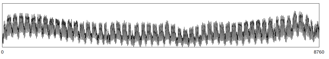
Fig. 15 Normalised electricity time series over the year.

Heating

We applied the same methodology as in previous paragraph to compute the residential, service heat yearly demand. The industrial heat processes demand is assumed to be the overall industrial energy demand where electricity and non energy use have been removed. Yearly EUD per sector is reported in table 1.4.

A part of the heat is assumed to be a fixed demand, such as hot water in households and services, or industrial processes. The other part represents the space heating demand and is varying. Similarly to the electricity, the ratio between varying electricity and fixed demand are the one of Switzerland, presented in ^2,5 which are based on ⁵². The varying demand of heat is shared over the year according to \(%_{sh}\). This time series is based on our own calculation. The methodology is the following: based on the temperature time series of Uccle 2015 (data from IRM ⁶⁰); the HDH are calculated; and then the time series. The HDH is a similar approach than the more commonly used HDD. According to Wikipedia, HDD is defined as follows: “HDD is a measurement designed to quantify the demand for energy needed to heat a building. HDD is derived from measurements of outside air temperature. The heating requirements for a given building at a specific location are considered to be directly proportional to the number of HDD at that location. […] Heating degree days are defined relative to a base temperature”. According to the European Environment Agency [37], the base temperature is 15.5\(^o\)C, we took 16\(^o\)C. HDH are computed as the difference between ambient temperature and the reference temperature at each hour of the year. If the ambient temperature is above the reference temperature, no heating is needed. Figure 16 compares the result of our methodology with real value collected by Eurostat [38]. The annual HDD was 2633, where we find 2507.

By normalising the HDH, we find \(%_{sh}\), which is represented in

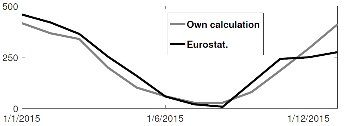
Fig. 16 Comparison of HDD between Eurostat and our own calculation.

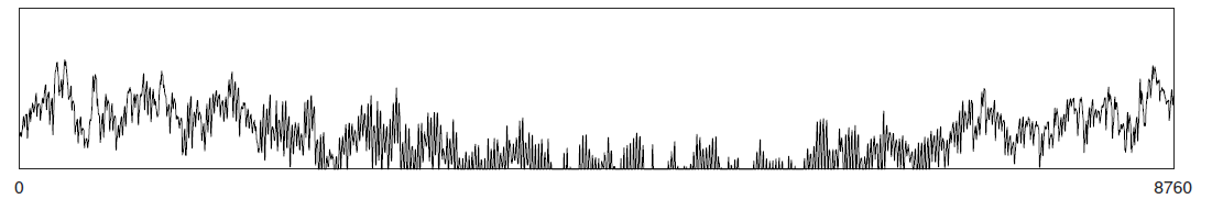
Fig. 17 Normalised space heating time series over the year.

Table 10 Yearly heat end use demand per sector, in 2035.

	Space heating	Hot water	Process heat [39]
	[TWh]	[TWh]	[TWh]
Households	70.2	18.0	0
Industry	13.1	3.4	50.4
Services	34.8	7.8	0

[39]

We define process heat as the high temperature heat required in the industrial processes. This heat cannot be supplied by technologies such as heat pumps or thermal solar.

Mobility

The annual passenger transport demand in Belgium for 2035 is expected to be 194 billions ²⁷. Passenger transport demand is divided between public and private transport. The lower (\(%_{public,min}\)) and upper bounds (\(%_{public,max}\)) for the use of public transport are 19.9% [40] and 50% of the annual passenger transport demand, respectively. The passenger mobility demand is shared over the day according to \(%_{pass}\). We assume a constant passenger mobility demand for every day of the year. This latter is represented in Figure Figure 18 (data from Figure 12 of ⁶¹). The annual freight transport demand in Belgium for 2035 is expected to be 98e09 tons kilometers ²⁷. The freight can be supplied by trucks, trains or boats. The lower (\(%_{fr,rail,min}\)) and upper bounds (\(%_{fr,rail,max}\)) for the use of freight trains are 10.9% and 25% of the annual freight transport demand, respectively. The lower (\(%_{fr,boat,min}\)) and upper bounds (\(%_{fr,boat,max}\)) for the use of freight inland boats are 15.6% and 30% of the annual freight transport demand, respectively. The lower (\(%_{fr,trucks,min}\)) and upper bounds (\(%_{fr,trucks,max}\)) for the use of freight trucks are 0% and 100% of the annual freight transport demand, respectively. The bounds and technologies information are latter summarised in Table 1.15.

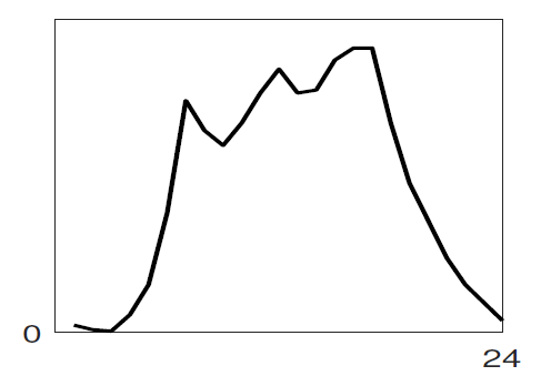
Fig. 18 Normalised passenger mobility time series over a day. We assume a similar passenger mobility demand over the days of the year.

Discount rate and interest rate

To compute their profitability, companies apply a discount rate to the investment they make. A discount rate is used for both cost of finance and for risk perception and opportunity cost. The cost of finance is to be compared with concepts like ‘hurdle rate’ or ‘rate of return’ usually calculated in accordance to an annual return on investment. Each individual investment physically occurring in year k, results in a stream of payments towards the amortization of this investment spread over several years in the future. The higher the cost of finance (or hurdle rate), the higher the annual payments spread over the lifetime of an investment and thus the higher the total cost. The hurdle rate affects only the investment costs so the impact is bigger for capital intensive technologies. We consider differentiated hurdle discount rates for different groups of energy supply and demand technologies, representing the different risk perception of industry versus individuals.

According with Meinke-Hubeny et al.⁶² who based their work on the JRC EU TIMES model ³⁷ in line with the PRIMES model ²⁷, the discount rate is around 7.5 up to 12% depending on the technologies. Discount rate cannot be directly converted into interest rate as the first is fixed by the market and the second is fixed by the central banks. As the evidence presented in Figure Figure 19 indicates, while these two interest rates tend to move together, they also may follow different paths from time to time.

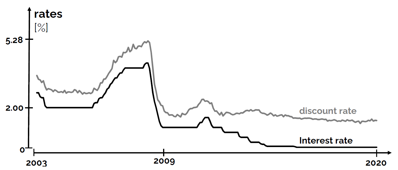
Fig. 19 Comparison of Belgian interest rate and discount rate. The following rate was chosen to represent the discount rate: floating loans rate over a 1M€ (other than bank overdraft) and up to 1 year initial rate fixation.

For the different studies, the real discount rate for the public investor \(i_{rate}\) is fixed to 1.5%, which is similar to the floating loan rate over a million euros (other than bank overdraft) and greater than the central bank interest rate.

Technologies

The technologies are regrouped by their main output types.

Electricity production

The following technologies are regrouped into two categories depending on the resources used: renewable or not.

Renewables

Table 11 Renewable electricity production technologies, in 2035. Abbreviations: onshore (on.), offshore (off.).

	\(c_ {inv}\)	\(c_ {maint}\)	\(gwp_ {constr}\)	\(li fetime\)	\(c_ {p}\)	\(f_ {min}\)	\(f_ {max}\)
	[€ 2015 /kW e]	[€ 2015 /kW e/y]	[kgCO 2-eq. /kW e]	[y]	[%]	[GW]	[GW]
Solar PV	870 [57]	18.8 [57]	2081 40	25 [57] 63	11.9 [58]	0	59.2 [59]
On. Wind Turbine	1040 [60]	12.1 [60]	622.9 40	30 [60] 64	24.3 [58]	0	10 [61]
Off. Wind Turbine	4975 [60]	34.6 [60]	622.9 40	30 [60] 64	41.2 [58]	0	6 [61]
Hydro River	5045 65	50.44 65	1263 40	40 65	48.4	0.38 66	0.38 66
Geothermal [63]	7488 [63]	142 [63]	24.9 40	30	86 67	0	0 [64]

[57] (1,2,3)

Investment cost based on ³⁵. OM cost scaled proportionally based on IEA data.

[58] (1,2,3)

Based on the real data of 2015 (data provided by ELIA, the Belgian TSO, which monitored 2952MW of PV, onshore and offshore in 2015 (Source: url{https://www.elia.be/}, consulted the 06/12/2019.})).

[59]

Assuming that 250 km\(^2\) of available roof well oriented exist today ⁴⁶ and that the efficiency in 2035 will be 23% ³⁵ with an average irradiation - similar to historical values - of 2820 Wh/m\(^2\) in Belgium, ³⁶. The upper limit becomes 59.2 GW of installed capacity.

[60] (1,2,3,4,5,6)

Onshore and offshore wind turbines in 2030 ³⁵. For Offshore, a correction factor of 2.58 is applied to have an LCOE of 79€/MWh in 2020, in line with recently published offer: https://www.enerdata.net/publications/daily-energy-news/belgium-agrees-79mwh-lcoe-three-offshore-wind-parks.html, visited on the 12-06-2020.

[61] (1,2)

From previous study ⁴⁴ with a correction on Offshore wind. The government announced a plan to build 6 GW of offshore wind, see Belgian offshore plateform.

[64]

A prototype (Balmatt project) started in 2019 and produces 4-5 MW ⁴⁷. However, the potential is not accurately known.

[63] (1,2,3)

ORC cycle at 6 km depth for electricity production. Based on Table 17 of ⁶⁸. We took the reference case in 2030.

Data for the considered renewable electricity production technologies are listed in Table 11, including the yearly capacity factor (\(c_p\)). As described in the Section [ssec:lp_formulation], for seasonal renewables the capacity factor \(c_{p,t}\) is defined for each time period. These capacity factors are represented in Figure Figure 20. For these technologies, \(c_p\) is the average of \(c_{p,t}\). For all the other electricity supply technologies (renewable and non-renewable), \(c_{p,t}\) is equal to the default value of 1. As the power delivered by the hydro river is almost negligible, we take the time series of hydro river from Switzerland ².

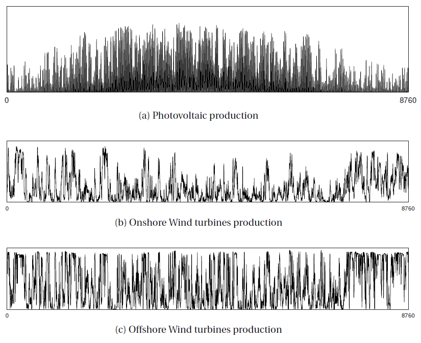
Fig. 20 Capacity factor for the different renewable energy sources over the year.

Non-renewable

Data for the considered fossil electricity production technologies are listed in Table 12. The maximum installed capacity (\(f_{max}\)) is set to a value high enough (100 000 TW_e) for each technology to potentially cover the entire demand.

Table 12 Non-renewable electricity supply technologies, in 2035. Abbreviations: Combined Cycles Gas Turbine (CCGT), Ultra-Supecritical (U-S), Integrated Gasification Combined Cycles (IGCC).

	\(c_ {inv}\)	\(c_ {maint}\)	\(gwp_ {constr}\)	\(li fetime\)	\(c_ {p}\)	\(\eta _e\)	\(C O_{2, direct}\) [81]
	[€ 2015 /kW e]	[€ 2015 /kW e/y]	[kgCO 2-eq. /kW e]	[y]	[%]	[%]	[tCO2/ MWh e ] [81]
Nuclear	4846 [82]	103 69	707.9 40	60 70	84.9 [83]	37	0
CCGT	772 69	20 69	183.8 40	25 71	85.0	63 [84]	0.317
CCGTAMMONIA [89]	772	20	183.8 40	25	85.0	50	0
Coal	2517 [85]	30 [85]	331.6 40	35 71	86.8 71	49 [86]	0.735
IGCC	3246 [87]	49 [87]	331.6 40	35 71	85.6 71	54 [88]	0.667

[81] (1,2)

Direct emissions due to combustion. Expressed in ton CO2 per MWh of electricity produced. Emissions computed based on resource used and specific emissions given in Table 8.

[82]

Investment cost: 3431 €₂₀₁₅/kW\(_{\text{e}}\) ⁶⁹ + dismantling cost in Switzerland: 1415 €₂₀₁₅/kW\(_{\text{e}}\) ⁷².

[83]

Data for the year 2012 ⁷³

[84]

0.4-0.5 GW\(_{e}\) CCGT in 2035 (realistic optimistic scenario) ⁷¹.

[85] (1,2)

1.3 GW\(_{e}\) advanced pulverized coal power plant ⁷⁴. cmaint is fixed cost (29.2 €₂₀₁₅/kW_e/y) + variable cost (0.51 €₂₀₁₅/kW_e/y assuming 7600 h/y).

[86]

Pulverized coal in 2025 (realistic optimistic scenario) ⁷¹.

[87] (1,2)

1.2 GW\(_{\text{e}}\) IGCC power plant ⁷⁴. cmaint is fixed cost (48.1 €₂₀₁₅/kW_e/y) + variable cost (0.82 €₂₀₁₅/kW_e/y assuming 7500 h/y).

[88]

IGCC in 2025 (realistic optimistic scenario) ⁷¹.

[89]

Use of Ammonia in CCGT is at its early stage. Mitsubishi is developping a 40 MW turbine and promises similar efficiency as gas CCGT ⁷⁵. However, the high emissions of NOx requires a removal equipment which will reduce the power plant efficiency. As gas and ammonia CCGT will be similar, we expect a similar cost and lifetime. The only exception is the efficiency, which is assumed at 50% instead of 63% for a gas CCGT ⁷⁶.

Heating and cogeneration

Tables 13, 14 and 15 detail the data for the considered industrial, centralized and decentralised CHP technologies, respectively. In some cases, it is assumed that industrial (Table 13) and centralized (:numref:` Table %s <tbl:dhn_cogen_boiler>`) technologies are the same. \(f_{min}\) and \(f_{max}\) for heating and CHP technologies are 0 and 100 TW_th, respectively. The latter value is high enough for each technology to supply the entire heat demand in its layer. the maximum (\(f_{max,\%}\)) and minimum (\(f_{min,\%}\)) shares are imposed to 0 and 100% respectively, i.e. they are not constraining the model.

Table 13 Industrial heating and cogeneration technologies, in 2035. Abbreviations: Combined Heat and Power (CHP), electricity (Elec.), Natural Gas (NG).

	\(c_ {inv}\)	\(c_ {maint}\)	\(gwp_ {constr}\)	\(li fetime\)	\(c_ {p}\)	\(\eta _e\)	\(\eta _{th}\)	\(C O_{2, direct}\)
	[€ 2015 /kW th]	[€ 2015 /kW th/y]	[kgCO 2-eq. /kW th]	[y]	[%]	[%]	[%]	[tCO2/ MWh th ] [115]
CHP NG	1408 [116]	92.6 [117]	1024 40	20 71	85	44 [118]	46 [118]	0.435
CHP Wood [119]	1080 69	40.5 69	165.3 40	25 77	85	18 69	53 69	0.735
CHP Waste	2928 [120]	111.3 [120]	647.8 [121]	25 77	85	20 77	45 77	0.578
Boiler NG	58.9 5	1.2 5	12.3 [122]	17 78	95	0	92.7 5	0.216
Boiler Wood	115 5	2.3 5	28.9 40	17 78	90	0	86.4 5	0.451
Boiler Oil	54.9 [123]	1.2 [124]	12.3 40	17 78	95	0	87.3 5	0.309
Boiler Coal	115 [125]	2.3 [125]	48.2 40	17 78	90	0	82	0.439
Boiler Waste	115 [125]	2.3 [125]	28.9 [126]	17 78	90	0	82	0.317
Direct Elec.	332 [127]	1.5 [127]	1.47 40	15	95	0	100	0

[115]

Direct emissions due to combustion. Expressed in ton CO2 per MWh of heat produced. Emissions computed based on resource used and specific emissions given in Table 8.

[116]

Calculated as the average of investment costs for 50 kW_e and 100 kW_e internal combustion engine cogeneration systems ⁵².

[117]

Calculated as the average of investment costs for 50 kW_e and 100 kW_e internal combustion engine cogeneration systems ⁷⁹.

[118] (1,2)

200 kW_e internal combustion engine cogeneration NG system, very optimistic scenario in 2035 ⁷¹.

[119]

Biomass cogeneration plant (medium size) in 2030-2035.

[120] (1,2)

Biomass-waste-incineration CHP, 450 scenario in 2035 ⁶⁹.

[121]

Impact of MSW incinerator in ⁵, using efficiencies reported in the table.

[122]

Assuming same impact as industrial oil boiler.

[123]

925 kW_th oil boiler (GTU 530) ⁸⁰

[124]

Assumed to be equivalent to a NG boiler.

[125] (1,2,3,4)

Assumed to be equivalent to a wood boiler.

[126]

Assuming same impact as industrial wood boiler.

[127] (1,2)

Commercial/public small direct electric heating ⁸¹.

Table 14 District heating technologies, in 2035. Abbreviations: biomass (bio.), CHP, digestion (dig.), hydrolysis (hydro.).

	\(c_ {inv}\)	\(c_ {maint}\)	\(gwp_ {constr}\)	\(li fetime\)	\(c_ {p}\)	\(\eta _e\)	\(\eta _{th}\)	\(C O_{2, direct}\)
	[€ 2015 /kW th]	[€ 2015 /kW th /y]	[kgCO 2 -eq./kW th]	[y]	[%]	[%]	[%]	[tCO2/ MWh th ] [154]
HP	345 [155]	12.0 [156]	174.8 40	25	95	0	400	0
CHP NG	1254 [157]	37.5 [157]	490.9 [158]	25 71	85	50 [159]	40 [159]	0.500
CHP Wood [160]	1081 69	40.5	165.3	25 77	85	18 69	53 69	0.736
CHP Waste [160]	2928	111	647.8	25 77	85	20 77	45 77	0.578
CHP bio. dig.	1374 [161]	147.9 [161]	647.8 [162]	25	85 [161]	13 [161]	16 [161]	2.488
CHP bio. hydro.	4537 [163]	227	647.8 [162]	15	85	25.4	33.5	1.164
Boiler NG	58.9 5	1.2	12.3	17 78	95	0	92.7 5	0.216
Boiler Wood	115 5	2.3 5	28.9	17 78	90	0	86.4 5	0.451
Boiler Oil	54.9	1.2	12.3	17 78	95	0	87.3 5	0.309
Geo thermal [165]	1500 [165]	57.0 [165]	808.8 40	30 [165]	85	0	100	0
Solar thermal [166]	362 [166]	0.43 [166]	221.8 40	30 [166]	10	0	100	0

[154]

Direct emissions due to combustion. Expressed in ton CO2 per MWh of heat produced. Emissions computed based on resource used and specific emissions given in :numref:` Table %s <tbl:prices_resources>`.

[155]

Calculated with the equation: cinv [EUR₂₀₁₁] = \(3737.6 * E^{0.9}\), where \(E\) is the electric power (kW_e) of the compressor, assumed to be 2150 kW_e. Equation from ⁸², taking only the cost of the technology (without installation factor).

[156]

Ground-water heat pump with 25 years lifetime ⁸³.

[157] (1,2)

CCGT with cogeneration ⁶⁹.

[158]

Impact of NG CHP in from ⁵, using efficiencies reported in the table.

[159] (1,2)

\(\eta\)_e and \(\eta\)_th at thermal peak load of a 200-250 MW_e CCGT plant, realistic optimistic scenario in 2035 ⁷¹.

[160] (1,2)

Assumed same technology as for industrial heat and CHP (Table 13)

[161] (1,2,3,4,5)

Cost estimations from ⁸⁴ and efficiencies from ⁸⁵. Data in line with IEA: ⁸⁶

[162] (1,2)

Construction emissions is assimilated to an industrial CHP waste technology.

[163]

Own calculation

[165] (1,2,3,4)

Geothermal heat-only plant with steam driven absorption heat pump 70/17\(^o\)C at 2.3 km depth (from ³⁵).

[166] (1,2,3,4)

Total system excluding thermal storage (from ³⁵).

Table 15 Decentralised heating and cogeneration technologies, in 2035. Abbreviations: Combined Heat and Power (CHP), electricity (Elec.), Fuel Cell (FC), Heat Pump (HP), Natural Gas (NG) and thermal (th.).

	\(c_ {inv}\)	\(c_ {maint}\)	\(gwp_ {constr}\)	\(li fetime\)	\(c_ {p}\)	\(\eta _e\)	\(\eta _{th}\)
	[€ 2015 /kW e]	[€ 2015 /kW e/y]	[kgCO 2 -eq./kW e]	[y]	[%]	[%]	[%]
HP	492 [207] [208]	21 [209]	164.9 40	18 [209]	100	0	300
Thermal HP	316 [210] [208]	9.5 [211]	381.9 40	20	100	0	150
CHP NG [212]	1408	92.6	1024	20 71	100	44	46
CHP Oil	1 306 [213]	82.0 [213]	1 024 [214]	20	100	39 [215]	43 [215]
FC NG	7 242 [216]	144.8 [217]	2193 40	20 87	100	58 [218]	22 [218]
FC H2 [219]	7242	144.8	2193	20 87	100	58	22
Boiler NG	159 5	5.08 5	4.8 5	17 78	100	0	90 5
Boiler Wood	462 88	16 88	2 1.1 [220]	17 78	100	0	85 88
Boiler Oil	142 80	8.5 [221]	21.15	17 78	100	0	85 5
Solar Th.	719 [222]	8.1 [223]	221.2 40	20 81	11.3[224]	0	NA
Direct Elec.	40 [225]	0 .18 [226]	1.47 40	15 81	100	0	100

[207]

10.9 kW_th Belaria compact IR heat pump ⁸⁹.

[208] (1,2)

Catalog data divided by 2.89. 2.89 is the ratio between Swiss catalog prices and prices found in the literature. Calculated by dividing the average price of a decentralised NG boiler (489 CHF₂₀₁₅/kW_th) in Swiss catalogs ⁹⁰ by the price for the equivalent technology found in literature (169 CHF₂₀₁₅/kW_th, from ⁵).

[209] (1,2)

6 kW_th air-water heat pump ⁸¹.

[210]

Specific investment cost for a 15.1 kW_th absorption heat pump (Vitosorp 200-F) ⁹⁰

[211]

3% of cinv (assumption).

[212]

Assumed same technology as for industrial CHP NG (Table 13)

[213] (1,2)

Assumed to be equivalent to a 100 kW_e internal combustion engine cogeneration NG system ^52,79.

[214]

Assuming same impact as decentralised NG CHP.

[215] (1,2)

Efficiency data for a 200 kW_e diesel engine ⁴⁰

[216]

System cost (including markup) for a 5 kW_e solid-oxide FC system, assuming an annual production of 50000 units ⁹¹.

[217]

2% of the investment cost ⁶⁹.

[218] (1,2)

Solid-oxide FC coupled with a NG turbine, values for very optimistic scenario in 2025 ⁸⁷.

[219]

Assumed to be equivalent to FC NG.

[220]

Assuming same impact as NG and oil decentralised boilers.

[221]

6% of cinv, based on ratio between investment and OM cost of boiler of similar size in ⁷⁸.

[222]

504 CHF₂₀₁₅/m\(^2\) for the UltraSol Vertical 1V Hoval system ⁸⁹. For conversion from €₂₀₁₅/m\(^2\) to €₂₀₁₅/kW_th, it is assumed an annual heat capacity factor of 6.5% based on Uccles data.

[223]

1.1% of the investment cost, based on ratio investment-to-OM cost in ⁸¹.

[224]

The calculation of the capacity factor for solar thermal is based on the IRM model ³⁶ with radiation data from the city of Uccles, Belgium.

[225]

Resistance heaters with fan assisted air circulation in ⁷⁸.

[226]

In the lack of specific data, same investment-to-OM ratio as for direct electric heating in the industry sector (Table 13).

Figure 21 represents the capacity factor (\(c_{p,t}\)) of solar thermal panels. The time series is the direct irradiation in Uccles in 2015, based on measurements of IRM. For all the other heat supply technologies (renewable and non-renewable) \(c_{p,t}\) is equal to the default value of 1.

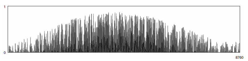
Fig. 21 Capacity factor of thermal solar panels over the year.

Transport

Passenger mobility

The vehicles available for passenger mobility are regrouped in two categories: public and private. Private accounts for all the cars owned (or rented) by the user, such as a gasoline car, a diesel car… In opposition to private, public mobility accounts for the shared vehicles. It accounts for buses, coaches, trains, trams, metro and trolleys. From the literature, data about mobility is not directly transposable to the model. Data about mobility are usually given per vehicles, such as a vehicle cost or an average occupancy per vehicle. These data are summarised in Table 16.

Table 16 Specific investment cost calculation based on vehicle investment data, in 2035. Abbreviations: average (av.), Fuel Cell (FC), Hybrid Electric Vehicle (HEV), Natural Gas (NG), Plug-in Hybrid Electric Vehicle (PHEV), public (pub.).

Vehicle type	\(Ve h.~Cost\)	\(Ma intenance\) [241]	\(Oc cupancy\)	\(Av. ~distance\)	\(Av. ~speed\)	\(li fetime\) [242]	\(gw p_{ constr}\)
		[k€\(_\ 2015\) /veh.]	[k€\(_\ 2015\) /veh./y]	[ pass/ veh.]	[1000 km/y]	[ km/h]	[ years]
Gasoline car	21 [243]	1.2	1.26 [244]	18 [245]	40	10	17.2
Diesel car	22 [243]	1.2	1.26 [244]	18 [245]	40	10	17.4
NG car	22 [243]	1.2	1.26 [244]	18 [245]	40	10	17.2
HEV car	22 [243]	1.74	1.26 [244]	18 [245]	40	10	26.2
PHEV car	23 [243]	1.82	1.26 [244]	18 [245]	40	10	26.2
BEV [246]	23 [243]	0.5	1.26 [244]	18 [245]	40	10	19.4
FC car	22 [243]	0.5	1.26 [244]	18 [245]	40	10	39.6
Tram and metro	2500	50.0	200	60	20	30	0 [247]
Diesel bus	220	11.0	24	39	15	15	0 [247]
Diesel HEV bus	300	12.0	24	39	15	15	0 [247]
NG bus	220	11.0	24	39	15	15	0 [247]
FC bus	375	11.3	24	39	15	15	0 [247]
Train pub.	10000	200.0	80	200	83	40	0 [247]

[241]

own calculation. The maintenance cost was assumed proportional to the investment cost and depending the type of powertrain. the average speed of private cars is calculated assuming that it is used 5% of the time (i.e. 1h12). Knowing the annual distance, the value is approximately 40 km/h.

[242]

In 2016, the average age of private cars was 8.9 years with a difference between regions ⁹².

[243] (1,2,3,4,5,6,7)

Costs are from mid-range vehicles estimation and projections of ⁹³.

[244] (1,2,3,4,5,6,7)

The federal bureau office estimates a decreasing average occupancy for cars down to 1.26 passenger/vehicle in 2030 ⁹⁴).

[245] (1,2,3,4,5,6,7)

In 2016, averaged yearly distance for private cars were between 9 500 and 21 100 kms depending on the type of powertrains, but in average around 18 000 kms.

[246]

Low range BEV have been implemented. Otherwise the investment cost is more than twice.

[247] (1,2,3,4,5,6)

No data found.

In Belgium, the car occupancy rate is less than 1.3 passengers per car: 1.3 in 2015 and estimated at 1.26 in ⁹⁴. The annual distance of a car depends on its type of motorization: from 9 500 km/year for a city gasoline car, to 21 100 km/year for a CNG one. On average, the distance is 18 000 km/year. The average age of a car is 8.9 years in 2016, with a variation between regions: in Brussels it is 10 years. On average, the distance is 18 000 km/year. The average age of a car is 8.9 years in 2016, with a rather strong variation between regions: in Brussels it is 10 years. Finally, a car drives on average a slightly more than one hour a day (1h12). Although private car usage habits may change, we extrapolate these data from today to future years. Certain trends, such as the mutualisation of a car, could lead to an increase in the annual distance travelled by a car. But other trends, such as autonomous cars, could lead to a further decrease in the car occupancy rate, to values below 1. These change may influence in both direction the specific price of a kilometer passenger provided by a car.

For public transportation, the data were collected from various report ^95,96,97. These data have been adapted based on discussion with experts in the field. They are reported in Table 16.

Surprisingly, in 2035, vehicles cost are similar regardless the power-train. Figure 22 shows how the vehicle cost vary over the transition, data from ⁹³. Today, we verify a strong price difference between the different technologies, this difference will diminish with the development of new technologies. The price difference between two technologies will become small as early as 2035 (\(\leq\)10%). In their work, National Research Council⁹³ estimates the cost of promising technologies in 2015 lower than the real market price. This is the case for BEV and FC vehicles, where the price ranges today around 60 k€₂₀₁₅ . These differences can be justified by three facts: these vehicles are usually more luxurious than others; The selling price do not represent the manufacturing cost for prototypes; the study is from 2013 and may have overestimated the production in 2015 and 2020.

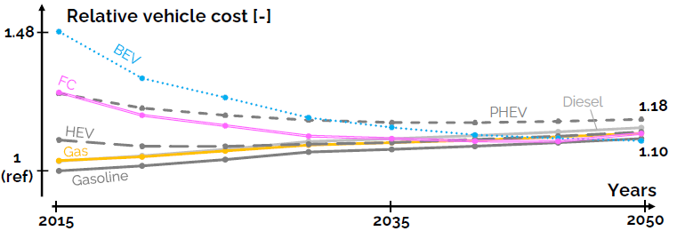
Fig. 22 Mid-range vehicle costs evolution during the transition. Reference (1.0 (ref)) is at 19.7 k€₂₀₁₅. Abbreviations: Carbon capture (CC), LFO, methanation (methan.), methanolation (methanol.), Natural Gas (NG), Synthetic Natural Gas (SNG), storage (sto.) and synthetic (syn.).

(44)\[c_{inv} (i) = \frac{vehicle~cost (i)}{occupancy (i)\cdot average~speed (i)} ~~~~~~ \forall i \in \text{TECH OF EUT} (PassMob)\]

(45)\[c_p = \frac{average~distance(i)}{average~speed(i)\cdot 8760} ~~~~~~ \forall i \in \text{TECH OF EUT} (PassMob)\]

(46)\[veh._{capa} (i) = occupancy (i)\cdot average~speed ~~~~~~ \forall i \in \text{TECH OF EUT} (PassMob)\]

From data of Table 16, specific parameters for the model are deduced. The specific investment cost (\(c_{inv}\)) is calculated from the vehicle cost, its average speed and occupancy, Eq. (44). The capacity factor (cp) is calculated based on the ratio between yearly distance and average speed, Eq. (45). The vehicle capacity is calculated based on the average occupancy and average speed, Eq. . (46). Table 17 summarises these information for each passenger vehicle.

An additional vehicle is proposed: methanol car. This choice is motivated to offer a zero emission fuels that could be competitve compared to electric or hydrogen vehicles. We assume that methanol is used through a spark-ignition engine in cars, and has similar performances than a gasoline car. This technology is added in the following tables.

Table 17 Passenger mobility financial information, in 2035 (based on data in Table 16). Abbreviations: Fuel Cell (FC), Hybrid Electric Vehicle (HEV), Natural Gas (NG), Plug-in Hybrid Electric Vehicle (PHEV), public (pub.).

Vehicle type	\(c_ {inv}\)	\(c_ {maint}\)	\(g wp_{ constr}\)	\(c_ p\)	\(V eh.~capa\)
[€/km -pass]	[€/km -pass/h]	[€/km -pass /h/y]	[kgCO2 -eq./km -pass/h]	[%]	[pass-km /h/veh.]
Gasoline car	420	24	342	5.1	50
Diesel car	434	24	346	5.1	50
NG car	429	24	342	5.1	50
HEV car	429	34	519	5.1	50
PHEV car	456	34	519	5.1	50
BEV	450	10	385	5.1	50
FC car	435	10	786	5.1	50
Methanol car [259]	420	24	342	5.1	50
Tram and metro	625	12.5	0 [250]	34.2	4000
Diesel bus	611	30.6	0 [250]	29.7	360
Diesel HEV bus	833	33.3	0 [250]	29.7	360
NG bus	611	30.6	0 [250]	29.7	360
FC bus	1042	31.3	0 [250]	29.7	360
Train pub.	1506	54.4	0 [250]	27.5	6640

[250] (1,2,3,4,5,6)

No data found

[259]

No data were found for methanol cars. Thus, we assume that the technology is similar to a gasoline car (except the fuel).

Table 18 summarises the forecast energy efficiencies for the different vehicles. For public vehicles in 2035, the energy efficiencies are calculated with a linear interpolation between the 2010 and 2050 values presented in Table 6 in Codina Gironès et al ⁹⁸. For private vehicles, Estimation for energy consumption for Belgium cars in 2030 are used ⁹⁴.

Table 18 Fuel and electricity consumption for passenger mobility technologies in 2035 ⁹⁸, and minimum/maximum shares allowed in the model. Abbreviations: Fuel Cell (FC), Hybrid Electric Vehicle (HEV), Natural Gas (NG), Plug-in Hybrid Electric Vehicle (PHEV), public (pub.).

Vehicle type	Fuel	Electricity	f\(_\textbf{min,%}\)	f\(_\textbf{max,%}\)
	[Wh/km-pass]	[Wh/km-pass]	[Wh/km-pass]	[%]
Gasoline car	497 [251]	0	0	1
Diesel car	435 [251]	0	0	1
NG car	543 [251]	0	0	1
HEV [252]	336 [251]	0	0	1
PHEV [253]	138 [251]	109 [251]	0	1
BEV	0	173 [251]	0	1
FC car	264 [254]	0	0	1
Methanol car	497 [251]	0	0	1
Tram & Trolley	0	63 [255]	0	0.17 [256]
Diesel bus	265	0	0	1
Diesel HEV bus	198	0	0	1
NG bus	268	0	0	1
FC bus	225	0	0	1
Train pub.	0	65 [255]	0	0.60 [256]

[251] (1,2,3,4,5,6,7,8)

calculation based on vehicle consumption in 2030 ⁹⁴ and occupancy of 2030 ⁹⁴. According to ⁹⁸, gas car are assumed to consume 25% more than diesel cars.

[252]

Using gasoline as only fuel.

[253]

It is assumed that electricity is used to cover 40% of the total distance and petrol to cover the remaining 60%.

[254]

In FC car are estimated to consume 52.6% more than BEV in 2035, see Table 2.12 in ⁹³

[255] (1,2)

Based on real data for the French case in 2004, from ⁹⁹. An increase of efficiency of 25% was assume.

[256] (1,2)

In 2015, the public mobility was shared as follow: trains (37.0%), trams/metros (8.7%) and buses (54.3%) ³². In 2035, we assume an upper limit twice greater than real data in 2015. Except for train were a maximum of 60% is imposed.

The size of the BEV batteries is assumed to be the one from a Nissan Leaf (ZE0) (24 kWh [257]). The size of the PHEV batteries is assumed to be the one from Prius III Plug-in Hybrid (4.4 kWh [258]). The performances of BEV and PHEV batteries are assimilated to a Li-ion battery as presented in Table 30. The state of charge of the electric vehicles (\(soc_{ev}\)) is constrained to 60% minimum at 7 am every days.

Freight mobility

The technologies available for freight transport are trains, trucks and boats. Similarly to previous section, the information for the freight is given per vehicles. These data are summarised in Table 19.

Table 19 Specific investment cost for freight vehicles, in 2035. Trucks data are from a report of 2019 ¹⁰⁰. Abbreviations: electric (elec.), Fuel Cell (FC) and Natural Gas (NG).

Vehicle type	\(Ve h.~Cost\)	\(Ma intenance\) [263]	\(To nnage\)	\(Av. ~distance\)	\(Av. ~speed\) [263]	\(li fetime\)
		[k€\(_ {2015}\) /veh.]	[k€\(_ {2015}\) /veh./y]	[ pass/ veh.]	[1000 km/y]	[ km/h]
Train freight [263]	4020	80.4	550	210	70	40
Boat Diesel [263]	2750	137.5	1200	30	30	40
Boat NG [263]	2750	137.5	1200	30	30	40
Boat Methanol	2750	137.5	1200	30	30	40
Truck Diesel	167	8.4	10	36.5 [264]	45	15
Truck FC	181	5.4	10	36.5	45	15
Truck Elec.	347	10.4	10	36.5	45	15
Truck NG	167	8.4	10	36.5	45	15

[263] (1,2,3,4,5)

Own calculation

[264]

In 2016, the average distance was between 16 974 up to 63 305 km per year depending on the truck category. Based on our own calculation, we found an average of 36 500 km per year.

Trucks have similar cost except for electric trucks. This last have a battery that supplies the same amount of kilometers than other technologies. As a consequence, half of the truck cost is related to the battery pack.

(47)\[c_{inv} (i) = \frac{vehicle~cost (i)}{tonnage (i)\cdot average~speed (i)} ~~~~~~ \forall i \in \text{TECH OF EUT} (FreightMob)\]

(48)\[c_p = \frac{average~distance(i)}{average~speed(i)\cdot 8760} ~~~~~~ \forall i \in \text{TECH OF EUT} (FreightMob)\]

(49)\[veh._{capa} (i) = tonnage (i)\cdot average~speed ~~~~~~ \forall i \in \text{TECH OF EUT} (FreightMob)\]

From Table 19, specific parameters for the model are deduced. Except for the technology construction specific GHG emissions (\(gwp_{constr}\)) where no data was found. The specific investment cost (cinv) is calculated from the vehicle cost, its average speed and occupancy, Eq. (47). The capacity factor (cp) is calculated based on the ratio between yearly distance and average speed, Eq. (48). The vehicle capacity is calculated based on the average occupancy and average speed, Eq. Eq. (49). Table 20 summarises these information for each freight vehicle.

Similarly to the methanol car, additional power trains have been added in order to open the competition between fuels and electric vehicles (including fuel cells electri vehicles). Methanol could be use with performances similar to the use of methane. Based on this approach, two technologies have been added: methanol boats and methanol trucks.

Table 20 Freight mobility financial information, in 2035. Abbreviations: electric (elec.), Fuel Cell (FC) and Natural Gas (NG).

Vehicle type	\(c_ {inv}\)	\(c_ {maint}\)	\(c_ p\)	\(V eh.~capa\)
	[€/km-t/h]	[€/km-t/h/y]	[%]	[t-km/h /veh.]
Train freight	104	2.1	34.2	38500
Boat Diesel	76	3.8	11.4	36000
Boat NG	76	3.8	11.4	36000
Boat Methnanol	76	3.8	11.4	36000
Truck Diesel	371	18.6	9.3	450
Truck FC	402	12.1	9.3	450
Truck Elec.	771	23.1	9.3	450
Truck NG	371	18.6	9.3	450
Truck Methanol	371	18.6	9.3	450

Trains and boats benefit on a very high tonnage capacity, and thus drastically reduce their specific investment cost down to 4-5 times lower than trucks. Table 20 summarises the forecast energy efficiencies for the different vehicles in 2035. Except for the technology construction specific GHG emissions (\(gwp_{constr}\)) where no data was found.

Table 21 Fuel and electricity consumption for freight mobility technologies, in 2035 ⁹⁸. Abbreviations: electric (elec.), Fuel Cell (FC) and Natural Gas (NG).

Vehicle type	Fuel	Electricity
	[Wh/km-t]	[Wh/km-t]
Train freight	0	68
Boat Diesel	107	0
Boat NG	123	0
Boat Diesel	107	0
Truck Diesel	513	0
Truck FC	440	0
Truck Elec.	0	249 [265]
Truck NG [266]	590	0
Truck Diesel	513	0

[265]

Energy intensity calculated based on the diesel one, and corrected with an electric to diesel powertrain ratio from ¹⁰⁰.

[266]

The efficiency is corrected with the ratio between NG bus and diesel bus.

Trains are considered to be only electric. Their efficiency in 2035 is 0.068 kWh/tkm ⁹⁸. The efficiency for freight transport by diesel truck is 0.51 kWh/tkm based on the weighted average of the efficiencies for the vehicle mix in ⁹⁸. For NG and H2 trucks, no exact data were found. Hence, we assume that the efficiency ratio between NG coaches and diesel coaches can be used for freight (same for H2 trucks). As a consequence, the efficiency of NG and H2 trucks are 0.59 and 0.44 kWh/tkm. Boats are considered to be diesel or gas powered. In 2015, the energy intensity ratio between diesel boats and diesel trucks were \(\approx\)20% [267]. By assuming a similar ratio in 2035, we find an efficiency of 0.107 kWh/tkm and 0.123 kWh/tkm for diesel and gas boats, respectively.

Non-energy demand

Non-energy demand plays a major role in the primary energy consumption in Belgium (20% in 2015, ⁴³). Rixhon et al.¹⁰¹ investigates the importance of non-energy demand worlwide and its projection based on the IEA reports (¹⁰²). Three main feedstocks have been chosen : ammonia, methanol and high-value chemicals (HVCs). This latter encompass different molecules, mainly hydrocarbons chains. Figure 23 illustrates the different conversion pathway to produce the different non-energy demand feedstocks.

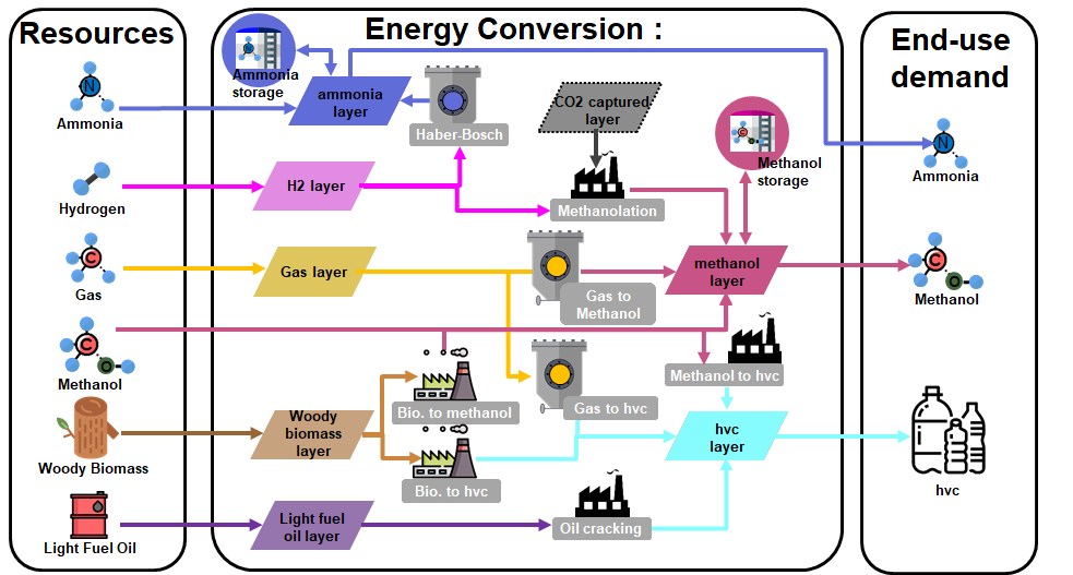
Fig. 23 Illustration of the technologies that produce non-energy feedstocks. For clarity, only the most relevant flows are drawn (Figure Figure 1 includes all the flows). Ammonia and methanol can be used in other sectors.

The Non-energy end-use demand is usuallty expressed in TWh/y without specifying the split among the feedstocks, such as the forecast used which are proposed by the European commission ²⁷. In Rixhon et al.¹⁰¹, they analysed the split among the three proposed feedstocks. In 2015, 77.9% of the NED accounted was for HVC, 19.2% for ammonia and only 2.9% for Methanol. Worlwide, the IEA forecast a similar growth for the different feedstocks (see Figure 4.5 of ¹⁰²). Thus, we assume a constant share between the three feedstocks.

Similarly to electricity, two of the three feedstocks can be used for other end-use demands. As an example, ammonia can be used for electricity production or methanol for mobility. Table 22 summarises the technology that produces HVC; Table 23 summarises the technology that produces methanol; and for ammonia, only the Haber-Bosch process is proposed in Table 24

Table 22 Production of High-Value Chemicals (HVCs) from different feedstocks, in 2035.

	\(c_ {inv}\)	\(c_ {maint}\)	\(life time\)	\(c_p\)	\(\eta_ {fuel}\)	\(\eta_ {e}\)	\(\eta_ {th,ht}\)	\(CO_ {2,direct}\) [359]
	[€\(_ {2015}\)/kW\(_ {fuel}\)]	[€\(_ {2015}\)/kW\(_ {fuel}\)/y]	[y]	[%]	[MWh/MWh\(_ {HVC}\)]	[MWh/MWh\(_ {HVC}\)]	[MWh/MWh\(_ {HVC}\)]	[tCO2 /MWhe]
Oil to HVC 103,104	395	2.1	15	100	1.82	0.021	0.017	0.213
Gas to HVC 105	798	20	25	100	2.79	0.47	0	0.299
Biomass to HVC 106	1743	52	20	100	2.38	0.029	0.052	0.669
Methanol to HVC 107,108	697	63	20	100	1.24	0	0.045	0.304

Table 23 Production of methanol from different feedstocks, in 2035.

	\(c_ {inv}\)	\(c_ {maint}\)	\(life time\)	\(c_p\)	\(\eta_ {fuel}\)	\(\eta_ {e}\)	\(\eta_ {th}\)	\(CO_ {2,direct}\) [359]
	[€\(_ {2015}\)/kW\(_ {fuel}\)]	[€\(_ {2015}\)/kW\(_ {fuel}\)/y]	[y]	[%]	[%]	[%]	[%]	[tCO2 /MWhe]
Biomass to methanol 109	2520	38.5	20	85	62	2	22	0.236
Syn. methanolation [361]	1680	84	20	67	0	0	26.1	-0.248
Methane to methanol 110 [362]	958.6	47.9	20	1	65.4	0	0	0.306

Table 24 Production of ammonia with the Haber Bosch process, in 2035. Data from Ikäheimo et al.⁷⁶.

	\(c_ {inv}\)	\(c_ {maint}\)	\(life time\)	\(c_p\)	\(\eta_ {fuel}\)	\(\eta_ {e}\)	\(\eta_ {th}\)	\(CO_ {2,direct}\) [359]
	[€\(_ {2015}\)/kW\(_ {fuel}\)]	[€\(_ {2015}\)/kW\(_ {fuel}\)/y]	[y]	[%]	[%]	[%]	[%]	[tCO2 /MWhe]
Haber bosch [364]	847	16.6	20	85	79.8 (NH3)	0	10.7	0

[364]

To produce 1 unit of ammonia, the system uses 1.13 units of H2 and 0.123 of electricity.

Synthetic fuels production

Synthetic fuels are expected to play a key role to phase out fossil fuels ¹¹¹. Figure 24 represents the technology related to synthetic fuels, including the CO2 layers. Synthetic fuels can be imported (Bio-ethanol, Bio-Diesel, H2 or SNG) or produced by converting biomass and/or electricity. The wet biomass - usually organic waste - can be converted through the biogas plant technology to SNG. This technology combines anaerobic digestion and cleaning processes. Woody biomass can be used to produce H2 through gasification, or different oils through pyrolysis or SNG through gasification to SNG. The different oil account for LFO, Gasoline or Diesel. The other processes to produce synthetic fuels are based on the water electrolysis, where the electrolysers convert electricity to H2. Then, the H2 can be combined with CO2 and upgraded to SNG through the methanation technology. In this latter, the process requires CO2. It can either be captured from large scale emitters, such as the industries and centralised heat technologies; or directly captured from the air but at a higher energetic and financial cost.

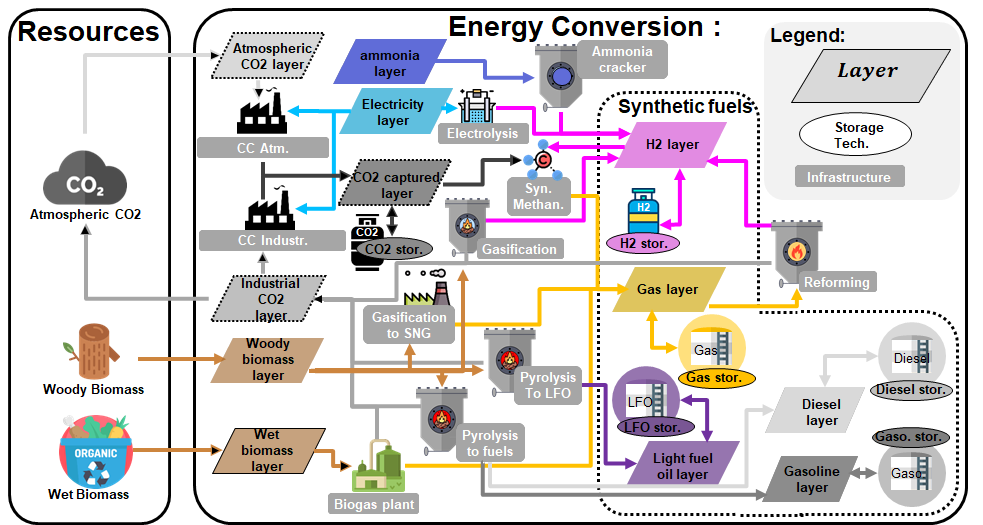
Fig. 24 Illustration of the technologies and processes to produce synthetic fuels. For clarity, only the most relevant flows are drawn (Figure Figure 1 includes all the flows). This Figure also illustrates how Carbon capture is implemented in the model. The CO:sub:2 emissions of large scale technologies can be either released at the atmosphere or captured by the Carbon Capture Industrial technolgy. Otherwise, CO:sub:2 can be captured from the atmosphere at a greater cost.

Hydrogen production

Three technologies are considered for hydrogen production: electrolysis, NG reforming and biomass gasification. The last two options can include CCS systems for limiting the CO\(_2\) emissions. They are Different technologies for electrolysis, in their work the Danish Energy Agency¹⁰⁹ review the PEM-EC, A-EC and SO-EC. Table 25 summarises the key characteristics for these technologies in year 2035.

Table 25 Characteristics of electrolyser technologies presented in ¹⁰⁹, in 2035. Efficiencies are represent as follow: Input (negative) and outputs (positive). Abbreviations: temperature (temp.), high temperature (h.t.), low temperature (l.t.), electricity (e), hydrogen (H2).

	\(c_ {inv}\)	\(c_ {maint}\)	\(life time\)	\(\eta_ e\)	\(\eta_ {h.t.}\)	\(\eta_ {H2}\)	\(\eta_ {l.t.}\)
	[€\(_ {2015}\)/kW\(_ {H2}\)]	[€\(_ {2015}\)/kW\(_ {H2}\)/y]	[y]	[%]	[%]	[%]	[%]
PEM-EC	870	40	15	-100		63	12
A-EC	806	43	25	-100		67	11
SO-EC	696	21	23	-85	-15	79	1.5

The different electrolyser cell technologies have a similar cost, however each technologies differ by their lifetime and electricity to hydrogen efficiencies. PEM-EC has the shortest lifetime and the lowest electricity to hydrogen efficiency, thus this technology will never be implemented in the model [335]. Electrolysers will be needed during excesses of electricity production, where heat demand is usually low. Thus, they aim at maximising the production of hydrogen rather than low temperature heat. For this reason, SO-EC appear as the most promising technology SO-EC appears as the most promising technology and will be implemented in the model. Thus, in this work, the term Electrolysis refers to SO-EC. Table 26 contains the data for the hydrogen production technologies.

Table 26 Hydrogen production technologies, in 2035.

	\(c_ {inv}\)	\(c_ {maint}\)	\(life time\)	\(c_p\)	\(\eta_ {H2}\)	\(CO_ {2,direct}\) [346]
	[€\({ _2015}\)/kW\(_ {H2}\)]	[€\({ _2015}\)/kW\(_ {H2}\)/y]	[y]	[%]	[%]	[tCO2 /MWhe]
Electrolysis [347] 109	696	21	23	90 [348]	79 [351]	0
NG reforming [349] 112	681	64.4	25	86	73	0.273
Biomass gasification [350] 112	2525	196	25	86	43	0.902
Ammonia cracking [352]	1365	38	25	85	59.1	0

[346]

Direct emissions due to combustion. Expressed in ton CO2 per MWh of fuel produced. Emissions computed based on resource used and specific emissions given in Table 8.

[347]

It uses electricity and high temperature heat as feedstock, see Table 25.

[348]

Own assumptions.

[349]

It uses gas as feedstock, such as NG.

[350]

It uses wood biomass as feedstock.

[351]

To produce one unit of H2, the system requires 1.076 units of electricity and 0.19 units of heat high temperature. We assume that, on top of the unit of H2 produced, an extra 0.019 units of low temperature heat can be recovered for district heating.

[352]

Cracking ammonia doesn’t exist at industrial scale. Indeed, ammonia is produced from hydrogen throuth the Haber-Bosch process. Thus, we didn’t found reliable data and did our own calculation based on Haber bosch process and methane cracking.

Synthetic methane and oils production

Three technology options are considered for the conversion of biomass to synthetic fuels: pyrolysis, gasification and biomethanation. The main product of the pyrolysis process is bio-oil. Two different pyrolysis process are thus proposed. One producing light fuel oil, and another one producing a blend of gasoline and diesel. The main product of the gasification and biomethanation processes are SNG, which is considered equivalent to gas. Data for the technologies are reported in Table 27 (from ⁵). The biomethanation process is based on anaerobic digestion followed by a cleaning process in order to have gas that can be reinjected in the gas grid ^109,113. In the table, efficiencies are calculated with respect to the wood in input (50% humidity, on a wet basis LHV) and ‘fuel’ stands for the main synthetic fuel in output. Finally, a last technology can produce methane from hydrogen and sequestrated CO:sub:2.

Table 27 Synthetic fuels (except H2) conversion technologies (from ^5,109 or specified), in 2035.

	\(c_ {inv}\)	\(c_ {maint}\)	\(life time\)	\(c_p\)	\(\eta_ {fuel}\)	\(\eta_ {e}\)	\(\eta_ {th}\)	\(CO_ {2,direct}\) [359]
	[€\(_ {2015}\)/kW\(_ {fuel}\)]	[€\(_ {2015}\)/kW\(_ {fuel}\)/y]	[y]	[%]	[%]	[%]	[%]	[tCO2 /MWhe]
Pyrolysis to LFO [363]	1344	67.2	25	85	66.6	1.58		0.586
Pyrolysis to fuels [363]	1365	38	25	85	57.4	1.58		0.586
Gasification	2525	178	25	85	65	0	22	0.260
Biomethanation [360]	986	88	25	85	29.9	0	0	0.722
Hydrolisis methanation 114	1592	112	15	100	42.3	0	4	0.306
Syn. methanation 115	280	0.21	30	86	83.3	0	0	-0.198

[359] (1,2,3,4)

Direct emissions due to combustion. Expressed in ton CO2 per MWh of fuel produced. Emissions computed based on resource used and produced and specific emissions given in Table 8.

[360]

Costs are adapted from ⁸⁴ and technical data from ⁸⁵.

[361]

Data from ¹¹⁶ to produce 1 MWh of methanol, the process requires 1.355 MWh of hydrogen and also 0.04 MWh of electricity, 0.107 MWh of heating and 0.210 units of cooling. The process is simplified to 1.5 MWh of hydrogen needed to produce 1 MWh of methanol.

[362]

This technology might be removed. Indeed, in this version of the model, synthetic liquid fuels are gathered together. However, they should be split in methanol, ethanol, bio-diesel… As a consequence, producing methanol from methane is cheaper than importing diesel. However in this version, methanol can be directly used as diesel \(\rightarrow\) a competitor.

[363] (1,2)

A distinction is made between pyrolysis to LFO and other fuels. The first can produce oil for heating or non-energy demand. The second produce a blend of diesel and gasoline (18% of gasoline and 39.4% of diesel).

Carbon capture and storage

As represented in Figure 24, two technologies are proposed to capture the CO2, one from atmosphere (CC atmospheric) and the other from exhaust gases of conversions processes (CC industry), such as after a coal power plant. Indeed, resources emit direct CO2 from combustion and CC industry can concentrate CO2 contained in the exhaust gas and inject it in CO2 captured layer. The same process can be performed at a higher energetical cost with CO2 from the atmosphere. No restriction on the available limit of CO2 from the atmosphere is considered. Data are summarised in Table 28.

We suppose that CC industry has similar characteristics than a sequestration unit on a coal power plant as proposed in ³⁵. Based on our own calculation, we evaluated the economical and technical data. We assumed that the energy drop of the power plant represents the amount of energy that the sequestration unit consumes. We assume that this energy must be supplied by electricity.

For CC atmospheric, Keith et al.¹¹⁷ proposed an installation where 1 ton of CO2 is captured from the atmosphere with 1.3 kWh of natural gas and electricity. We assume that it can be done with 1.3 kWh of electricity. The thermodynamical limit is estimated to be around 0.2 kWh of energy to sequestrate this amount ¹¹⁸.

Table 28 Carbon capture (CC) technologies, in 2035. \(E_e\) represents the electricity required to capture sequestrate CO2. \(\eta_{CO_2}\) represents the amount of CO2 sequestrated from the CO2 source. Abbreviations: industrial (ind.), atmospheric (atm.).

	\(c_ {inv}\)	\(c_ {maint}\)	\(life time\)	\(E_e\)	\(\eta_ {CO_2}\)	\(f_ {min,\%}\)	\(f_ {max,\%}\)
	[€\(_ {2015}\)/kW\(_ {fuel}\)]	[€\(_ {2015}\)/kW\(_ {fuel}\)/y]	[y]	[kWh:sub`e`/ tCO2]	[%]	[%]	[%]
CC Ind.	2580	64.8	40	0.233	90 [367]	0	100
CC Atm.	5160 [368]	129.6	40	1.3	100	0	100

[367]

We consider that 10% of the CO2 cannot be collected.

[368]

Based on the economical data given in ¹¹⁷ and own calculation.

No relevant data were found for the capacity factor (\(\textbf{c}_\textbf{p}\)) and the GWP associated to the unit construction.

Storage

Tables 29 and 30 detail the data for the storage technologies. Table 29 summarises the investment cost, GWP, lifetime and potential integration of the different technologies. Table 30 summarises the technical performances of each technology.

Table 29 Storage technologies characteristics in 2035: costs, emissions and lifetime. Abbreviations: batteries (batt.), Battery Electric Vehicule (BEV), centralised (cen.), decentralised (dec.), Lithium-ions (Li-on), Natural Gas (NG), Plug-in Hybrid Electric Vehicle (PHEV), Pumped Hydro Storage (PHS), seasonal (seas.), temperature (temp.) and thermal storage (TS).

	\(c_ {inv}\)	\(c_ {maint}\)	\(gw p_{con str}\)	\(li fetime\)
	[\(\ €_{2015}\) /kWh]	[\(\ €_{2015}\) /kWh/y]	[kgCO2 -eq./kWh]	[y]
Li-on batt.	302 [294]	0.62 [294]	61.3 [295]	15 [296]
PHS	58.8	0 [297]	8.33 [298]	50 [299]
TS dec.	19.0 [300]	0.13 [300]	0 [297]	25 [300]
TS seas. cen.	0.54 [301]	0.003 [301]	0 [297]	25 [301]
TS daily cen.	3 [301]	0.0086 [301]	0 [297]	40 [300]
TS high temp.	28	0.28	0 [297]	25
Gas	0.051 [302]	0.0013 [302]	0 [297]	30 [302]
H2	6.19 [303]	0.03 [303]	0 [297]	20 [303]
Diesel [304]	6.35e-3	3.97e-4	0 [297]	20
Gasoline [304]	6.35e-3	3.97e-4	0 [297]	20
LFO [304]	6.35e-3	3.97e-4	0 [297]	20
Ammonia [304]	6.35e-3	3.97e-4	0 [297]	20
Methanol [304]	6.35e-3	3.97e-4	0 [297]	20
CO2 [305]	49.5 [306]	0.495	0 [297]	20

[294] (1,2)

We assume a Lithium-ion NMC battery at a utility-scale in 2030 ¹¹⁹ with average use of 100 cycles/year.

[295]

Data from Table 4 of ⁴⁴.

[296]

Trade off between various sources: ^119,120

[297] (1,2,3,4,5,6,7,8,9,10,11,12,13)

Neglected.

[298]

Own calculation based on Hydro Dams emissions from previous work ^2,5.

[299]

Data verified in Table B1 of ¹²⁰.

[300] (1,2,3,4)

Adapted from Table 5.2 of ¹²¹.

[301] (1,2,3,4,5)

The technologies used are pit thermal energy storage technology and Large-scale hot water tanks for seasonal and daily DHN storage, respectively. Data was taken for year 2030 ¹¹⁹.

[302] (1,2,3)

Data from the Torup Lille project ¹¹⁹. The lifetime is assumed similar to a cavern for hydrogen storage.

[303] (1,2,3)

Based on tank storage from the JRC project:cite:simoes2013jrc. The cost is assumed as the average of 2020 and 2050 costs.

[304] (1,2,3,4,5)

In this implementation, the power of fuel imported can be constrained to be constant among the year. Thus, a storage is created for the fuel, even if the storage cost is negligeable (see Eq. (41)). Data were obtained by our own calculation.

[305]

Based on liquid CO2 tank storage. Data from a datasheet of Ever grow gas company https://www.evergrowgas.com/. Lifetime and maintenance cost based on own calculation.

[306]

Units: cinv [€₂₀₁₅/tCO₂], cop [€₂₀₁₅/tCO₂/y]

The PHS in Belgium can be resumed to the Coo-Trois-Ponts hydroelectric power station. The characteristics of the station in 2015 are the following: installed capacity turbine (1164MW), pumping (1035MW), overall efficiency of 75%, all reservoirs capacity (5000 MWh). We assume that the energy losses is shared equally between the pumping and turbining, resulting by a charge/discharge efficiencies of 86.6%. The energy to power ratio are 4h50 and 4h18 for charge and discharge, respectively ¹²². A project started to increase the height of the reservoirs and thus increase the capacity by 425 MWh. In addition, the power capacity will be increase by 80MW. The overall project cost is estimated to 50M€ and includes also renovation of other parts [307]. We arbitrary assume that 50% is dedicated for the height increase. It results in an investment cost of 58.8€₂₀₁₅ per kWh of new capacity. The overall potential of the PHS could be extended by a third reservoir with an extra capacity of around 1.2 GWh. Hence, we assume that the upper limit of PHS capacity is 6.5 GWh. No upper bound were constrained for other storage technologies.

Estimation for the gas storage is based on an existing facility using salt caverns as reservoirs: Lille Torup in Danemark ¹¹⁹. The project cost is estimated to 254M€₂₀₁₅ for an energy capacity of 4965 GWh. The yearly operating cost is estimated to 6.5 M€₂₀₁₅. Part of it is for electricity and gas self consumption. We assume that the electricity is used for charging the system (compressing the gas) and the gas is used for heating up the gas during the discharge. These quantities slightly impact the charge and discharge efficiency of the system. The charge and discharge power are 2200 and 6600 [MW] respectively. As the technology is mature, we assume that the cost of the technology in 2035 will be similar to Lille Torup project.

Table 30 Storage technologies characteristics in 2035: efficiencies, energy to power ratios, losses and availabilities. Abbreviations: batteries (batt.), Battery Electric Vehicule (BEV), centralised (cen.), decentralised (dec.), Lithium-ions (Li-on), Natural Gas (NG), Plug-in Hybrid Electric Vehicle (PHEV), Pumped Hydro Storage (PHS), seasonal (seas.), temperature (temp.) and thermal storage (TS).

	\(\eta_ {sto,in}\)	\(\eta_ {sto,out}\)	\(t_ {sto,in}\)	\(t_ {sto,out}\)	\(%_ {sto_{loss}}\)	\(%_ {sto_{avail}}\)
	[-]	[-]	[h]	[h]	[s\(^ {-1}\)]	[-]
Li-on batt.	0.95 [326]	0.95 [326]	4 [326]	4 [326]	2e-4 [326] [327]	1
BEV batt.	0.95 [326]	0.95 [326]	4 [328]	10 [328]	2e-4 [326] [327]	0.2 [328]
PHEV batt.	0.95 [326]	0.95 [326]	4 [328]	10 [328]	2e-4 [326] [327]	0.2 [328]
PHS	0.866	0.866	4.30	4.83	0 [329]	1
TS dec.	1 [329]	1 [329]	4 [328]	4 [328]	82e-4 [330]	1
TS seas. cen.	1 [331]	1 [331]	150 [331]	150 [331]	6.06e-5 [331]	1
TS daily cen.	1 [331]	1 [331]	60.3 [331]	60.3 [331]	8.33e-3 [331]	1
TS high temp.	1 [331]	1 [331]	2	2	3.55e-4 [331]	1
NG	0.99 [332]	0.995 [332]	2256 [332]	752 [332]	0	1
H2	0.90 [333]	0.98 [333]	4 [333]	4 [333]	0	1
Diesel [334]	1	1	168	168	0	1
Gasoline [334]	1	1	168	168	0	1
LFO [334]	1	1	168	168	0	1
Ammonia [334]	1	1	168	168	0	1
Methanol [334]	1	1	168	168	0	1
CO2	1	1	1	1	0	1

[326] (1,2,3,4,5,6,7,8,9,10,11)

Data verified in Table B1 of ¹²⁰.

[327] (1,2,3)

Data from Table 4 of ⁴⁴.

[328] (1,2,3,4,5,6,7,8)

Own calculation.

[329] (1,2,3)

Neglected.

[330]

Adapted from Table 5.2 of ¹²¹

[331] (1,2,3,4,5,6,7,8,9,10,11,12,13)

Based on the Pit thermal energy storage technology in 2030 for seasonal and Large-scale hot water tanks for DHN daily storage. Data from ¹¹⁹.

[332] (1,2,3,4)

Data from the Torup Lille project:cite:DanishEnergyAgency2018. Efficiencies are based on our own calculation based on electricity and gas consumed by the installation over a year.

[333] (1,2,3,4)

Sadaghiani and Mehrpooya¹²³ an efficiency of 88.6% in an ideal configuration for liquid hydrogen liquefaction. This high efficiency is used and we arbitrary impose that the charge efficiency is 90% and the discharge 98%. The tank design by JRC ³⁷ has a charge/discharge energy to power ratio of 4 hours.

[334] (1,2,3,4,5)

We assume a perfect storage with 1 week of charge/discharge time.

Others

Electricity grid

No data were found for the Belgian grid. Hence, by assuming that the grid cost is proportional to the population, the Belgian grid cost can be estimated based on the known Swiss grid cost. In 2015, the population of Belgium and Switzerland were 11.25 and 8.24 millions, respectively (Eurostat). The replacement cost of the Swiss electricity grid is 58.6 billions CHF₂₀₁₅ ¹²⁴ and its lifetime is 80 years ¹²⁵. The electricity grid will need additional investment depending on the penetration level of the decentralised and stochastic electricity production technologies. The needed investments are expected to be 2.5 billions CHF₂₀₁₅ for the high voltage grid and 9.4 billions CHF₂₀₁₅ for the medium and low voltage grid. This involves the deployment of 25GW of PV and 5.3 GW of wind onshore. These values correspond to the scenario 3 in ¹²⁴. The lifetime of these additional investments is also assumed to be 80 years.

By assuming a linear correlation between grid reinforcement and intermittent renewable deployment, the specific cost of integration is estimated to 393 MCHF per GW of renewable intermittent energy installed (\((9.4+2.5)\)bCHF\(/(25+5.3)GW = 0.393\)bCHF/GW) .

As a consequence, the estimated cost of the Belgian grid is \(58.6/1.0679\cdot 11.25/8.24=74.9\) b€₂₀₁₅. And the extra cost is \(393/1.0679\approx 367.8\) M€₂₀₁₅/GW.

Belgium is strongly interconnected to neighbouring countries. Based on an internal report of the TSO ¹²⁶, the TTC is estimated to be 6500 GW in 2020, which is in line with another study from EnergyVille ⁶² and the ENTSOE ¹²⁷. However, the NTC published by the TSO on his website is much lower, around 3100 MW: 950 MW from Netherlands, 1800 MW from France and 350 MW from England (in 2020). This NTC is defined as ‘The net transfer capacity (NTC) is the forecast transfer capacity agreed by Elia and its neighbouring transmission system operators (TSOs) for imports and exports across Belgium’s borders. […] EU Regulation 543/2013 refers to net transmission capacity as ‘forecasted capacity’.’ [369]. As explained in an internal report of the TSO ¹²⁸, the TTC is an upper bound of the NTC. In the literature, studies analysing the Belgium energy system accounts for the TTC, thus this capacity was implemented in this work: 6500 MW in 2020. The ENTSOE published his Ten Year Network Development Plan for different periods up to 2040. They estimates, if all projects are commissionned before 2035, the cross border capacities in 2035 up to 14 780 MW, which represents more than twice the available capacity in 2020 ¹²⁷. Figure 25 illustrates the capacity changes for each neighbouring country, interconnections are reinforced in every countries more or less proportionally to the existing capacities.

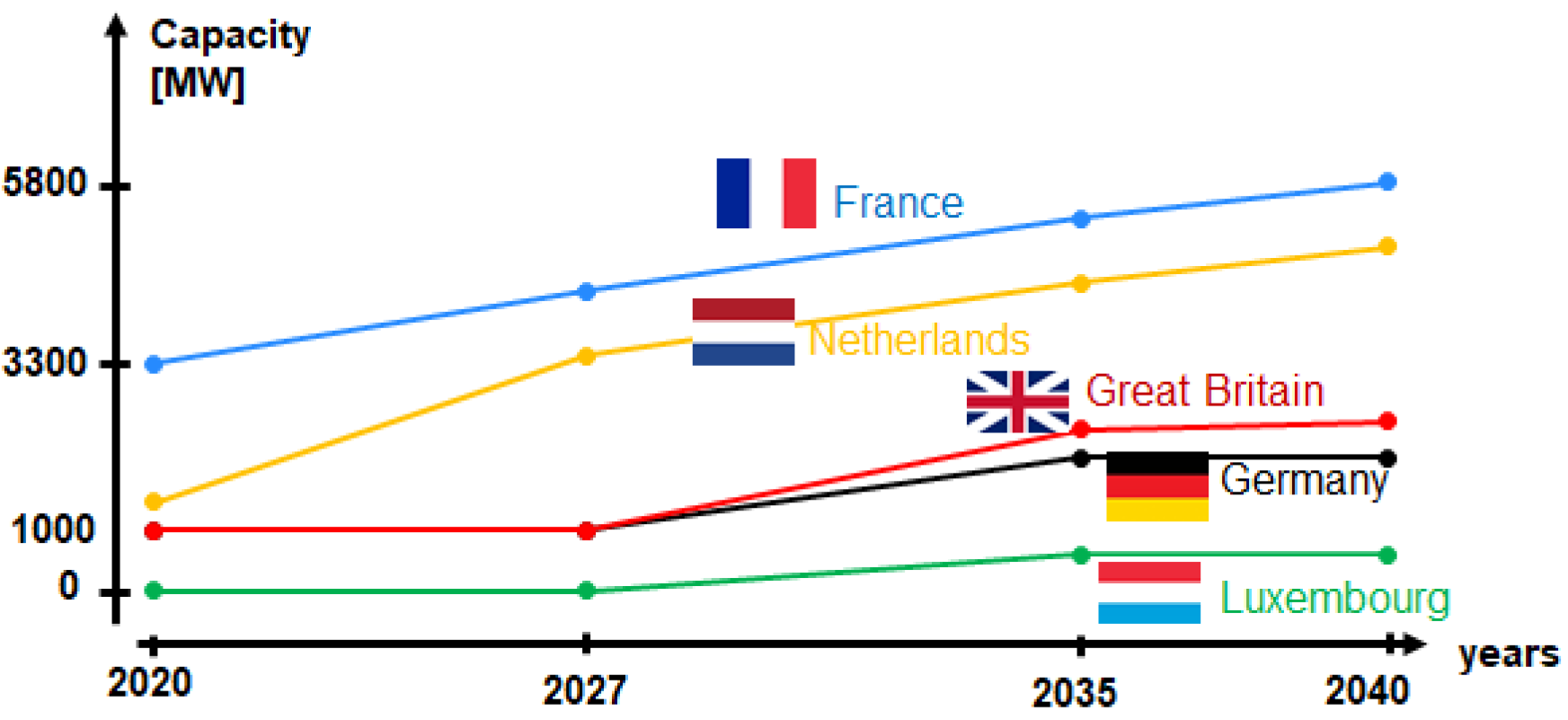
Fig. 25 Expected capacities between Belgium and neighbouring countries. Data from ¹²⁷.

Losses (\(\%_{\emph{net\textsubscript{loss}}}\)) in the electricity grid are fixed to 4.7%. This is the ratio between the losses in the grid and the total annual electricity production in Belgium in 2016 ³².

In a study about “electricity scenarios for Belgium towards 2050´´, the TSO estimates the overall import capacity up to 9.88 GW ⁴⁵. The interconnections are built as follow: 3.4 GW from Netherlands, 4.3 GW from France, 1.0 GW from Germany, 1.0 GW from Great Britain and 0.18 GW from Luxembourg [370]. However, a maximum simultaneous import capacity is fixed to 6.5 GW and justified as follow “Additionally, the total maximum simultaneous import level for Belgium is capped at 6500 MW. For a relatively small country with big and roughly adequate neighbours, the simulations show that a variable import volume up to the maximum of 6500 MW can happen, thanks to the non-simultaneousness of peaks between the countries. But during certain hours, there is not enough generation capacity abroad due to simultaneous needs in two or more countries which will result in a lower import potential for Belgium. This effect is taken into account in the model´´ ⁴⁵. The same ratio of simultaneous import and NTC (66%) is used for the other years.

Losses (\(%_{net_{loss}}\)) in the electricity grid are fixed to 4.7%. This is the ratio between the losses in the grid and the total annual electricity production in Belgium in 2016 ³².

DHN grid

For the DHN, the investment for the network is also accounted for. The specific investment (\(c_{inv}\)) is 882 CHF₂₀₁₅/kW_th in Switzerland. This value is based on the mean value of all points in ¹²⁹ (Figure 3.19), assuming a full load of 1535 hours per year (see table 4.25 in ¹²⁹). The lifetime of the DHN is expected to be 60 years. DHN losses are assumed to be 5%.

As no relevant data were found for Belgium, the DHN infrastructure cost of Switzerland was used. As a consequence, the investment cost (\(c_{inv}\)) is 825 €₂₀₁₅/kW_th. Based on the heat roadmap study ¹³⁰, heat provided by DHN is “around 2% of the heating for the built environment (excluding for industry) today to at least 37% of the heating market in 2050”. Hence, the lower (%dhn,min) and upper bounds (%dhn,max) for the use of DHN are 2% and 37% of the annual low temperature heat demand, respectively.

Energy demand reduction cost

By replacing former device at the end user side, the EUD can be reduced. This is usually called an ‘energy efficiency’ measure. As an example, by insulating a house, the space heating demand can be reduced. However, energy efficiency has a cost which represents the extra cost to reduce the final energy needed to supply the same energy service. As in the model the demand reduction is fixed, hence the energy efficiency cost is fixed. The American Council for an Energy-Efficient Economy summarises study about the levelised cost of energy savings ¹³¹. They conclude that this cost is below 0.04 USD₂₀₁₄/kWh saved and around 0.024 USD₂₀₁₄/kWh, hence 0.018€₂₀₁₅/kWh. In 2015, Belgium FEC was 415 TWh ⁴³ and the energy efficiency around 15% compare to 1990. The European target is around 35% in 2035, hence the energy efficiency cost for Belgium between 2015 and 2035 is 3.32b€₂₀₁₅. This result is in line with another study for Switzerland where the energy efficiency cost is 1.8b€₂₀₁₅ for the same period and similar objectives ¹³² (see ⁵ for more details about Switzerland).

[1]

The database is consulted online: http://www.ecoinvent.org

[2]

Real values are expressed at the net of inflation. They differ from nominal values, which are the actual prices in a given year, accounting for inflation.

[9]

250 km\(^2\) represents almost a hundredth of Belgium’s land area, which is 28635 km\(^2\). The total area, accounting for water areas, of Belgium is 30528 km\(^2\). From https://fr.wikipedia.org/wiki/G%C3%A9ographie_de_la_Belgique, visited the 10/08/2020.

[10]

A similar calculation was done for solar thermal with an efficiency of 28%.

[11]

In the study, potential are given in PetaJoules of electricity per year (58-185 PJ for onshore and 8-10 PJ for offshore) for EROI of 5 and 12 (see Table 13 of ). To convert energy into power capacity, capacity factors of 24% and 41% for onshore and offshore, were assumed respectively.

[37] (1,2)

From https://www.eea.europa.eu/data-and-maps/indicators/heating-degree-days-2, consulted the 06-12-2019

[38]

Source: https://ec.europa.eu/eurostat, consulted the 06/12/2019.

[40]

it corresponds to the share of 2015 (From Tables 2.2.3 and 2.3.3 of ³²), in line with data from the SPF ¹³³.

[257]

from https://en.wikipedia.org/wiki/Nissan_Leaf, consulted on 29-01-2019

[258]

from https://fr.wikipedia.org/wiki/Toyota_Prius, consulted on 29-01-2019

[267]

Value calculated based on the ratio between the transported tons and the consumed energy per technologies in 2015. Data from ²⁷

[307]

This information was shared by Engie, the facility manager https://corporate.engie-electrabel.be/projet-extension-centrale-coo/ and also publicised by newspapers: https://www.renouvelle.be/fr/actualite-belgique/la-centrale-de-coo-augmente-sa-capacite-de-stockage, https://www.lameuse.be/403176/article/2019-06-20/va-agrandir-les-lacs-de-la-centrale-coo.

[335]

Not all the characteristics of the cell has been implemented, thus PEM-EC can be competitive compare to other technologies.

[369]

Information and definition from the TSO website: https://www.elia.be/en/grid-data/transmission/yearly-capacity, visited on the 29th of May 2020

[370]

More details about capacities and projects are given in Figure 56 of ⁴⁵.