Model formulation

Model overview:

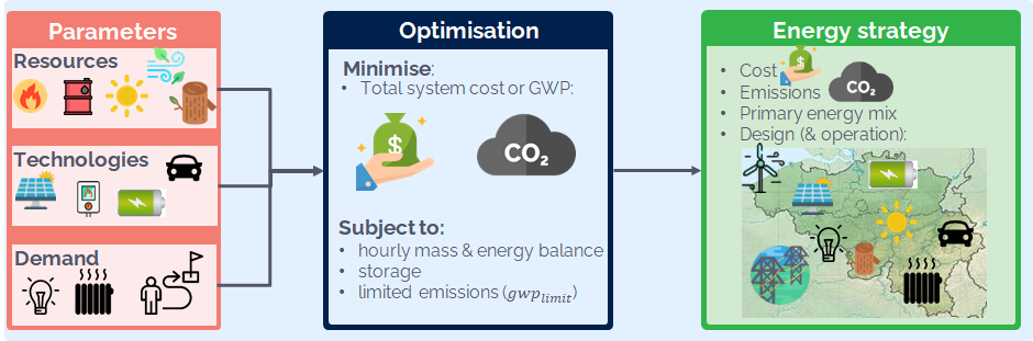
Fig. 3 Overview of the LP modeling framework.

Overview

Due to computational restrictions, energy system models rarely optimise the 8760h of the year. As an example, running our model with 8760h time series takes more than 19 hours; while the hereafter presented methodology needs approximately 1 minute. A typical solution is to use a subset of representative days called TD; this is a trade-off between introducing an approximation error in the representation of the energy system (especially for short-term dynamics) and computational time.

• the first step consists in pre-processing the time series and solving a MILP problem to determine the adequate set of (Section Typical days selection).

• the second step is the main energy model: it identifies the optimal design and operation of the energy system over the selected (Section Energy system model), i.e. technology selection, sizing and operation for a target future year.

These two steps can be computed independently. Usually, the first step is computed once for an energy system with given weather data whereas the second step is computed several times (once for each different scenario). The following Figure 4 illustrates the overall structure of the code.

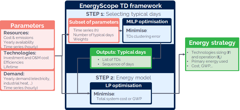
Fig. 4 Overview of the EnergyScope TD framework in two-steps. STEP 1: optimal selection of typical days (Section Typical days selection). STEP 2: Energy system model (Section Energy system model). The first step processes only a subset of parameters, which account for the 8760h time series. Abbreviations: TD, MILP, LP and GWP

This documentation is built from previous works (^1,2,5). For more details about the research approach, the choice of clustering method or the reconstruction method; refer to ¹.

Typical days selection

Resorting to TDs has the main advantage of reducing the computational time by several orders of magnitude. Usually, studies use between 6 and 20 TDs ^18,19,20,21 sometimes even less ^22,23.

Clustering methods

In a previous work ², it has been estimated that 12 typical days were appropriate for this model. Moreover, a comparison between different clustering algorithm shown that the method of ²³ had the best performances.

Caution

A small mistake has been corrected on the distance used in the clustering method. The impact of this mistake on previous work has been assessed and the conclusion is that the impact is negligible. The error and explanation are detailed in the pdf Erratum_STEP_1.pdf.

Implementing seasonality with typical days

Using TDs can introduce some limitations. As an example, traditionally, model based on TDs are not able to include inter-days or seasonal storage due to the discontinuity between the selected days. Thus, they assess only the capacity of production without accounting for storage capacities. Carbon-neutral energy system will require long term storage and thus, this limitation must be overcome. Therefore, we implemented a method proposed by Gabrielli et al.¹⁸ to rebuild a year based on the typical days by defining a sequence of . This allows to optimise the storage level of charge over the 8760h of the year. Gabrielli et al.¹⁸ assigned a TD to each day of the year; all decision variables are optimised over the TDs, apart from the amount of energy stored, which is optimised over 8760h. This methodology is illustrated in the follwing Figure 5.

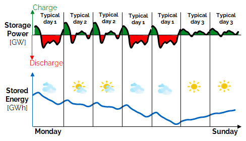
Fig. 5 Illustration of the typical days reconstruction method proposed by ¹⁸ over a week. The example is based on 3 TDs: TD 1 represents a cloudy weekday, applied to Monday, Thursday and Friday; TD 2 is a sunny weekday, applied to Tuesday and Wednesday; and TD 3 represents sunny weekend days. The power profile (above) depends solely on the typical day but the energy stored (below) is optimised over the 8760 hours of the year (blue curve). Note that the level of charge is not the same at the beginning (Monday 1 am) and at the end of the week (Sunday 12 pm).

The performances of this method has been quantified in a previous work ². With 12 Typical days, the key performances indicators (cost, emissions, installed capacity and primary energy used) are well captured. The only exception are the long term storage capacities which are slightly underestimated (by maximum a factor of 2).

Energy system model

Hereafter, we present the core of the energy model. First, we introduce the conceptual modelling framework with an illustrative example, in order to clarify as well the nomenclature. Second, we introduce the constraints of the energy model (data used are detailed in the Section Input Data).

Linear programming formulation

The model is mathematically formulated as a LP problem ²⁴. Figure 6 represents - in a simple manner - what is a LP problem and the nomenclature used. In italic capital letters, SETS are collections of distinct items (as in the mathematical definition), e.g. the RESOURCES set regroups all the available resources (NG, WOOD, etc.). In italic lowercase letters, parameters are known values (inputs) of the model, such as the demand or the resource availability. In bold with first letter in uppercase, Variables are unknown values of the model, such as the installed capacity of PV. These values are determined (optimised) by the solver within an upper and a lower bound (both being parameters). As an example, the installed capacity of wind turbines is a decision variable; this quantity is bounded between zero and the maximum available potential. Decision variables can be split in two categories: independent decision variables, which can be freely fixed, and dependent decision variables, which are linked via equality constraints to the previous ones. As an example the investment cost for wind turbines is a variable but it directly depends on the number of wind turbines, which is an independent decision variable. Constraints are inequality or equality restrictions that must be satisfied. The problem is subject to (s.t.) constraints that can enforce, for example, an upper limit for the availability of resources, energy or mass balance, etc. Finally, an objective function is a particular constraint whose value is to be maximised (or minimised).

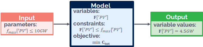
Fig. 6 Conceptual illustration of a LP problem and the nomenclature used. Symbol description: maximum installed size of a technology (fmax), installed capacity of a technology (F) and total system cost (Ctot). In this example, a specific technology (F [’PV’]) has been chosen from the set TECHNOLOGY.

Conceptual modelling framework

The proposed modelling framework is a simplified representation of an energy system accounting for the energy flows within its boundaries. Its primary objective is to satisfy the energy balance constraints, meaning that the demand is known and the supply has to meet it. In the energy modelling practice, the energy demand is often expressed in terms of FEC. According to the definition of the European commission, FEC is defined as “the energy which reaches the final consumer’s door” ²⁵. In other words, the FEC is the amount of input energy needed to satisfy the EUD in energy services. As an example, in the case of decentralised heat production with a NG boiler, the FEC is the amount of NG consumed by the boiler; the EUD is the amount of heat produced by the boiler, i.e. the heating service needed by the final user.

The input for the proposed modelling framework is the EUD in energy services, represented as the sum of four energy-sectors: electricity, heating, mobility and non-energy demand; this replaces the classical economic-sector based representation of energy demand. Heat is divided in three EUTs: high temperature heat for industry, low temperature for space heating and low temperature for hot water. Mobility is divided in two EUTs: passenger mobility and freight [1]. Non-energy demand is, based on the IEA definition, “fuels that are used as raw materials in the different sectors and are not consumed as a fuel or transformed into another fuel.” ²⁶. As examples, the European Commission includes as non-energy the following materials: “chemical feed-stocks, lubricants and asphalt for road construction.” ²⁷.

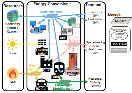
Fig. 7 Conceptual example of an energy system with 3 resources, 8 technologies (of which 2 storages (in colored oval) and 1 infrastructure (grey rectangle)) and 3 end use demands. Abbreviations: PHS, electrical heat pump (eHP), CHP, CNG. Some icons from ²⁸.

A simplified conceptual example of the energy system structure is proposed in Figure 7. The system is split in three parts: resources, energy conversion and demand. In this illustrative example, resources are solar energy, electricity and NG. The EUD are electricity, space heating and passenger mobility. The energy system encompasses all the energy conversion technologies needed to transform resources and supply the EUD. In this example, Solar and NG resources cannot be directly used to supply heat. Thus, they use technologies, such as boilers or CHP for NG, to supply the EUT layer (e.g. the high temperature industrial heat layer). Layers are defined as all the elements in the system that need to be balanced in each time period; they include resources and EUTs. As an example, the electricity layer must be balanced at any time, meaning that the production and storage must equal the consumption and losses. These layers are connected to each other by technologies. We define three types of technologies: technologies of end-use type, storage technologies and infrastructure technologies. A technology of end-use type can convert the energy (e.g. a fuel resource) from one layer to an EUT layer, such as a CHP unit that converts NG into heat and electricity. A storage technology converts energy from a layer to the same one, such as TS that stores heat to provide heat. In this example ( Figure 7), there are two storage technologies: TS for heat and PHS for electricity. An infrastructure technology gathers the remaining technologies, including the networks, such as the power grid and DHNs, but also technologies linking non end-use layers, such as methane production from wood gasification or hydrogen production from methane reforming.

As an illustrative example of the concept of layer, Figure Figure 8 gives a perspective of the electricity layer which is the most complex one, since the electrification of other sectors is foreseen as a key of the energy transition ²⁹. In the proposed version, 42 technologies are related to the electricity layer. 9 technologies produce exclusively electricity, such as CCGT, PV or wind. 12 cogenerations of heat and power (CHPs) produce heat and electricity, such as industrial waste CHP. 6 technologies are related to the production of synthetic fuels and CCS. 1 infrastructure represents the grid. 4 storage technologies are implemented, such as PHS, batteries or V2G. The remains are consumers regrouped in the electrification of heat and mobility. Electrification of the heating sector is supported by direct electric heating but also by the more expensive but more efficient electrical heat pumps for low temperature heat demand. Electrification of mobility is achieved via electric public transportation (train, trolley, metro and electrical/hybrid buses), electric private transportation including and hydrogen cars [2] and trains for freight.

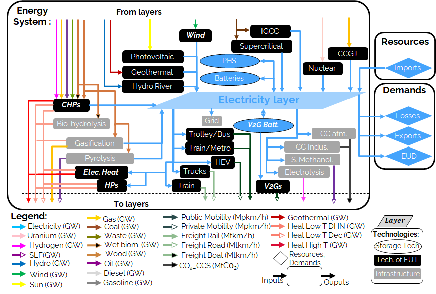
Fig. 8 Representation of the Electricity layer with all the technologies implemented in ESTD v2.1. Bold Italic technologies represent a group of different technologies. Abbreviations: atmospheric (atm.), Carbon capture (CC), CCGT, CHP, HP, electricity (elec.), HP, industrial (ind.) IGCC, PHS, synthetic methanolation (S. Methanol.), V2G, EUD.

The energy system is formulated as a LP problem. It optimises the design by computing the installed capacity of each technology, as well as the operation in each period, to meet the energy demand and minimize the total annual cost of the system. In the following, we present the complete formulation of the model in two parts. First, all the terms used are summarised in a figure and tables: Figure 9 for sets, Tables 1 and 2 for parameters, and 3 and 4 for variables. On this basis, the equations representing the constraints and the objective function are formulated in Figure 10 and Eqs. (1) - (39) and described in the following paragraphs.

Sets, parameters and variables

Figure 9 gives a visual representation of the sets with their relative indices used in the followings. 1 and 2 list and describe the model parameters. Tables 3 and 4 list and describe the independent and dependent variables, respectively.

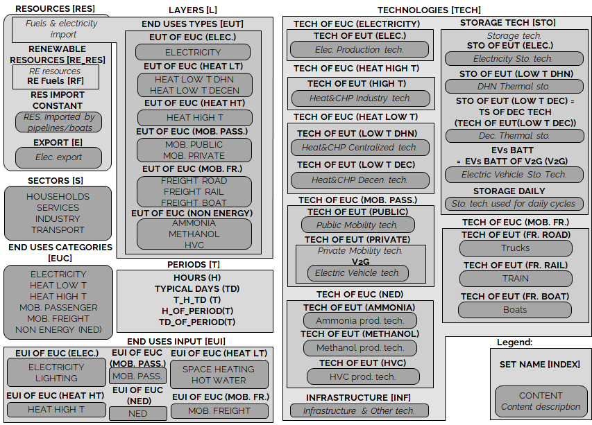
Fig. 9 Visual representation of the sets and indices used in the LP framework. Abbreviations: SH, HW, temperature (T), MOB, passenger (Pass.), V2G, TS.

Table 1 Time series parameters

Parameter	Units	Description
\(\%_{elec}(h,td)\)	[-]	Yearly time series (adding up to 1) of electricity end-uses
\(\%_{sh}(h,td)\)	[-]	Yearly time series (adding up to 1) of SH end-uses
\(\%_{elec}(h,td)\)	[-]	Yearly time series (adding up to 1) of passenger mobility end-uses
\(\%_{fr}(h,td)\)	[-]	Yearly time series (adding up to 1) of freight mobility end-uses
\(c_{p,t}(tech,h,td)\)	[-]	Hourly maximum capacity factor for each technology (default 1)

Table 2 List of parameters (except time series).

Parameter	Units	Description
\(\tau\)(tech)	[-]	Investment cost annualization factor
\(i_{rate}\)	[-]	Real discount rate
\(endUses_ {year} (eui,s)\)	[GWh/y] [a]	Annual end-uses in energy services per sector
\(endUsesInput (eui)\)	[GWh/y] [a]	Total annual end-uses in energy services
\(re_{share}\)	[-]	minimum share [0;1] of primary RE
\(gwp _{limit}\)	[ktCO\(_{2-eq}\)/y]	Higher CO\(_{2-eq}\) emissions limit
\(\%_ {public,min}, \%_{public,max}\)	[-]	Lower and upper limit to \(\textbf{%}_ {\textbf{Public}}\)
\(\%_ {fr,rail,min}, \%_{fr,rail,max}\)	[-]	Lower and upper limit to \(\textbf{%}_ {\textbf{Fr,Rail}}\)
\(\%_ {fr,boat,min}, \%_{fr,boat,max}\)	[-]	Lower and upper limit to \(\textbf{%}_ {\textbf{Fr,Boat}}\)
\(\%_ {fr,truck,min}, \%_{fr,truck,max}\)	[-]	Lower and upper limit to \(\textbf{%}_ {\textbf{Fr,Truck}}\)
\(\%_ {dhn,min}, \%_{dhn,max}\)	[-]	Lower and upper limit to \(\textbf{%}_ {\textbf{Dhn}}\)
\(\%_ {ned}(EUT\_OF\_EUC( NON\_ENERGY))\)	[-]	Share of non-energy demand per type of feedstocks
\(t_ {op}(h,td)\)	[h]	Time period duration (default 1h)
\(f_{min}, f_{max} (tech)\)	[GW] [a] [b]	Min./max. installed size of the technology
\(f_{min,\%}, f_{max,\%}(tech)\)	[-]	Min./max. relative share of a technology in a layer
\(avail(res)\)	[GWh/y]	Resource yearly total availability
\(c_{op}(res)\)	[M€\(_{2015}\)/GWh]	Specific cost of resources
\(veh_{capa}\)	[km-pass/h/veh.] [a]	Mobility capacity per vehicle (veh.).
\(\%_{ Peak_{sh}}\)	[-]	Ratio peak/max. space heating demand in typical days
\(f( res\cup tech \setminus sto, l)\)	[GW] [c]	Input from (<0) or output to (>0) layers . f(i,j) = 1 if j is main output layer for technology/resource i.
\(c_ {inv}(tech)\)	[M€\(_{2015}\) /GW] [c] [b]	Technology specific investment cost
\(c_{maint} (tech)\)	[M€\(_{2015}\) /GW/y] [c] [b]	Technology specific yearly maintenance cost
\({ lifetime}(tech)\)	[y]	Technology lifetime
\(gwp_{constr} (tech)\)	[ktCO\(_2\)-eq./GW] [a] [b]	Technology construction specific GHG emissions
\(gwp_ {op}(res)\)	[ktCO\(_2\)-eq./GWh]	Specific GHG emissions of resources
\(c_{p}(tech)\)	[-]	Yearly capacity factor
\(\eta_{s to,in},\eta_{sto ,out} (sto,l)\)	[-]	Efficiency [0;1] of storage input from/ output to layer. Set to 0 if storage not related to layer
\(\%_{ sto_{loss}}(sto)\)	[1/h] (self discharge)	Losses in storage
\(t_{sto_{in}} (sto)\)	[-]	Time to charge storage (Energy to power ratio)
\(t_{sto_{out}} (sto)\)	[-]	Time to discharge storage (Energy to power ratio)
\(\%_ {sto_{avail}} (sto)\)	[-]	Storage technology availability to charge/discharge
\(\%_{net_ {loss}}(eut)\)	[-]	Losses coefficient \([0;1]\) in the networks (grid and DHN)
\(ev_{b att,size}(v2g)\)	[GWh]	Battery size per V2G car technology
\(soc_{min,ev} (v2g,h)\)	[GWh]	Minimum state of charge for electric vehicles
\(c_ {grid,extra}\)	[M€\(_2015\)/GW]	Cost to reinforce the grid per GW of intermittent renewable
\(elec_{ import,max}\)	[GW]	Maximum net transfer capacity
\({solar}\) _ \({area}\)	[km\(^2\)]	Available area for solar panels
\({power}\) _ \(density_{pv}\)	[GW/km\(^2\)]	Peak power density of PV
\({power}\) _ \(density_{ solar,thermal}\)	[GW/km\(^2\)]	Peak power density of solar thermal

[a] (1,2,3,4,5)

[Mpkm] (millions of passenger-km) for passenger, [Mtkm] (millions of ton-km) for freight mobility end-uses

[b] (1,2,3,4)

[GWh] if \({{tech}} \in {{STO}}\)

[c] (1,2,3)

[Mpkm/h] for passenger, [Mtkm/h] for freight mobility end-uses

Table 3 Independent variables. All variables are continuous and non-negative, unless otherwise indicated.

Variable	Units	Description
\(\textbf{%}_{ \textbf{Public}}\)	[-]	Ratio \([0;1]\) public mobility over total passenger mobility
\(\textbf{%}_{ \textbf{Fr,Rail}}\)	[-]	Ratio \([0;1]\) rail transport over total freight transport
\(\textbf{%}_{ \textbf{Fr,Boat}}\)	[-]	Ratio \([0;1]\) boat transport over total freight transport
\(\textbf{%}_{ \textbf{Fr,Truck}}\)	[-]	Ratio \([0;1]\) truck transport over total freight transport
\(\textbf{%}_{ \textbf{Dhn}}\)	[-]	Ratio \([0;1]\) centralized over total low-temperature heat
\(\textbf{F}(tech)\)	[GW] [d]	Installed capacity with respect to main output
\(\textbf{F}_ {\textbf{t}}(tech \cup res,h,td)\)	[GW] [d]	Operation in each period
\(\textbf{Sto}_{ \textbf{in}}, \textbf{Sto}_{ \textbf{out}} (sto, l, h, td)\)	[GW]	Input to/output from storage units
\(\textbf{P}_{ \textbf{Nuclear}}\)	[GW]	Constant load of nuclear
\(\textbf{Import}_ \textbf{Constant}\) (RES_IMPORT_CONSTANT)	[GW]	Resources imported at a constant flow
\(\textbf{%}_{ \textbf{PassMob}}(TECH\ OF\ EUC(PassMob))\)	[-]	Constant share of passenger mobility
\(\textbf{%}_{ \textbf{FreightMob}} (TECH~OF~EUC(FreightMob))\)	[-]	Constant share of freight mobility
\(\textbf{%}_{ \textbf{HeatLowTDEC}} (TECH~OF~EUT(HeatLowTDec) \setminus {Dec_{Solar}} )\)	[-]	Constant share of low temperature heat decentralised supplied by a technology plus its associated thermal solar and storage
\(\textbf{F}_{ \textbf{sol}} (TECH~OF~EUT(HeatLowTDec) \setminus {Dec_{Solar}})\)	[-]	Solar thermal installed capacity associated to a decentralised heating technology
\(\textbf{F}_{ \textbf{t}_{\textbf{sol}}} (TECH~OF~EUT(HeatLowTDec) \setminus {Dec_{Solar}})\)	[-]	Solar thermal operation in each period

[d] (1,2)

[Mpkm] (millions of passenger-km) for passenger, [Mtkm] (millions of ton-km) for freight mobility end-uses

Table 4 Dependent variable. All variables are continuous and non-negative, unless otherwise indicated.

Variable	Units	Description
\(\textbf{ EndUses}(l,h,td)\)	[GW] [e]	End-uses demand. Set to 0 if \(l \notin\) EUT
\(\textbf{C}_ {\textbf{tot}}\)	[M€2015/y]	Total annual cost of the energy system
\(\textbf{C}_ {\textbf{inv}}( tech)\)	[M€2015]	Technology total investment cost
\(\textbf{C}_ {\textbf{maint}}( tech)\)	[M€2015/y]	Technology yearly maintenance cost
\(\textbf{C}_ {\textbf{op}}( res)\)	[M€2015/y]	Total cost of resources
\(\textbf{GWP}_ {\textbf{tot}}\)	[ktCO\(_2\)-eq./y]	Total yearly GHG emissions of the energy system
\(\textbf{GWP}_ {\textbf{constr}}( tech)\)	[ktCO\(_2\)-eq.]	Technology construction GHG emissions
\(\textbf{GWP}_ {\textbf{po}}( res)\)	[ktCO\(_2\)-eq./y]	Total GHG emissions of resources
\(\textbf{Net}_ {\textbf{losses}}( eut,h,td)\)	[GW]	Losses in the networks (grid and DHN)
\(\textbf{Sto}_ {\textbf{level}}( sto,t)\)	[GWh]	Energy stored over the year

[e]

[Mpkm] (millions of passenger-km) for passenger, [Mtkm] (millions of ton-km) for freight mobility end-uses

Energy model formulation

In the following, the overall LP formulation is proposed through Figure 10 and equations  (1) - (42) the constraints are regrouped in paragraphs. It starts with the calculation of the EUD. Then, the cost, the GWP and the objective functions are introduced. Then, it follows with more specific paragraphs, such as storage or vehicle-to-grid implementations.

End-use demand

Imposing the EUD instead of the FEC has two advantages. First, it introduces a clear distinction between demand and supply. On the one hand, the demand concerns the definition of the end-uses, i.e. the requirements in energy services (e.g. the mobility needs). On the other hand, the supply concerns the choice of the energy conversion technologies to supply these services (e.g. the types of vehicles used to satisfy the mobility needs). Based on the technology choice, the same EUD can be satisfied with different FEC, depending on the efficiency of the chosen energy conversion technology. Second, it facilitates the inclusion in the model of electric technologies for heating and transportation.

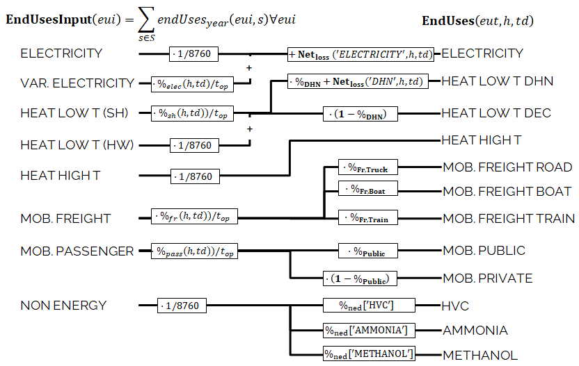
Fig. 10 Hourly EndUses demands calculation starting from yearly demand inputs (endUsesInput). Adapted from ⁵. Abbreviations: space heating (sh), district heating network (DHN), high value chemicals (HVC), hot water (HW), passenger (pass), freight (fr) and non-energy demand (NED).

The hourly end-use demands (EndUses) are computed based on the yearly end-use demand (endUsesInput), distributed according to its time series (listed in Table 1). Figure 10 graphically presents the constraints associated to the hourly end use demand (EndUses), e.g. the public mobility demand at time \(t\) is equal to the hourly passenger mobility demand times the public mobility share (%Public).

Electricity end-uses result from the sum of the electricity-only demand, assumed constant throughout the year, and the variable demand of electricity, distributed across the periods according to %elec. Low-temperature heat demand results from the sum of the yearly demand for HW, evenly shared across the year, and SH, distributed across the periods according to %sh. The percentage repartition between centralized (DHN) and decentralized heat demand is defined by the variable %Dhn. High temperature process heat and mobility demand are evenly distributed across the periods. Passenger mobility demand is expressed in passenger-kilometers (pkms), freight transportation demand is in ton-kilometers (tkms). The variable %Public defines the penetration of public transportation in the passenger mobility sector. Similarly, %Rail, %Boat and %Truck define the penetration of train, boat and trucks for freight mobility, respectively.

Cost, emissions and objective function

(1)\[\text{min} \textbf{C}_{\textbf{tot}} = \sum_{j \in \text{TECH}} \Big(\textbf{$\tau$}(j) \textbf{C}_{\textbf{inv}}(j) + \textbf{C}_{\textbf{maint}} (j)\Big) + \sum_{i \in \text{RES}} \textbf{C}_{\textbf{op}}(i)\]

(2)\[\begin{split}\text{s.t. } \textbf{$\tau$}(j) = \frac{i_{\text{rate}}(i_{\text{rate}}+1)^{lifetime(j)}}{(i_{\text{rate}}+1)^{lifetime(j)} - 1} ~~~~~~ \forall j \in \text{TECH}\\\end{split}\]

(3)\[\begin{split}\textbf{C}_{\textbf{inv}}(j) = c_{\text{inv}}(j) \textbf{F}(j) ~~~~~~ \forall j \in \text{TECH}\\\end{split}\]

(4)\[\begin{split}\textbf{C}_{\textbf{maint}}(j) = c_{\text{maint}}(j) \textbf{F}(j) ~~~~~~ \forall j \in \text{TECH}\\\end{split}\]

(5)\[\textbf{C}_{\textbf{op}}(i) = \sum_{t \in T | \{h,td\} \in T\_H\_TD(t)} c_{\text{op}}(i) \textbf{F}_{\textbf{t}}(i,h,td) t_{op} (h,td) ~~~~~~ \forall i \in \text{RES}\]

The objective, Eq. (1), is the minimisation of the total annual cost of the energy system (\(\textbf{C}_{\textbf{tot}}\)), defined as the sum of the annualized investment cost of the technologies (\(\tau\textbf{C}_{\textbf{inv}}\)), the operating and maintenance cost of the technologies (\(\textbf{C}_{\textbf{maint}}\)) and the operating cost of the resources (\(\textbf{C}_{\textbf{op}}\)). The total investment cost (\(\textbf{C}_{\textbf{inv}}\)) of each technology results from the multiplication of its specific investment cost (\(c_{inv}\)) and its installed size (F), the latter defined with respect to the main end-uses output [3] type, Eq. (3). \(\textbf{C}_{\textbf{inv}}\) is annualised with the factor \(\tau\), calculated based on the interest rate (\(t_{op}\)) and the technology lifetime (lifetime), Eq. (2). The total operation and maintenance cost is calculated in the same way, Eq. (4). The total cost of the resources is calculated as the sum of the end-use over different periods multiplied by the period duration (\(t_{op}\)) and the specific cost of the resource (\(c_{op}\)), Eq. (5). Note that, in Eq. (5)), summing over the typical days using the set T_H_TD [4] is equivalent to summing over the 8760h of the year.

(6)\[ \begin{align}\begin{aligned}\textbf{GWP}_\textbf{tot} = \sum_{j \in \text{TECH}} \frac{\textbf{GWP}_\textbf{constr} (j)}{lifetime(j)} + \sum_{i \in \text{RES}} \textbf{GWP}_\textbf{op} (i)\\\left(\text{in this version of the model} : \textbf{GWP}_\textbf{tot} = \sum_{i \in \text{RES}} \textbf{GWP}_\textbf{op} (i) \right)\end{aligned}\end{align} \]

(7)\[\textbf{GWP}_\textbf{constr}(j) = gwp_{\text{constr}}(j) \textbf{F}(j) ~~~~~~ \forall j \in \text{TECH}\]

(8)\[\textbf{GWP}_\textbf{op}(i) = \sum_{t \in T| \{h,td\} \in T\_H\_TD(t)} gwp_\text{op}(i) \textbf{F}_\textbf{t}(i,h,td) t_{op} (h,td )~~~~~~ \forall i \in \text{RES}\]

The global annual GHG emissions are calculated using a LCA approach, i.e. taking into account emissions of the technologies and resources ‘from cradle to grave’. For climate change, the natural choice as indicator is the GWP, expressed in ktCO\(_2\)-eq./year. In Eq. (6), the total yearly emissions of the system (\(\textbf{GWP}_{\textbf{tot}}\)) are defined as the sum of the emissions related to the construction and end-of-life of the energy conversion technologies \(\textbf{GWP}_{\textbf{constr}}\), allocated to one year based on the technology lifetime (\(lifetime\)), and the emissions related to resources \(\textbf{GWP}_{\textbf{op}}\)). Similarly to the costs, the total emissions related to the construction of technologies are the product of the specific emissions (\(gwp_{constr}\) and the installed size (\(\textbf{F}\)), Eq. (7). The total emissions of the resources are the emissions associated to fuels (from cradle to combustion) and imports of electricity (\(gwp_{op}\)) multiplied by the period duration (\(t_{op}\)), Eq. (8). GWP accounting can be conducted in different manners deepending on the scope of emission. The European Commission and the IEA mainly uses resource-related emissions \(\textbf{GWP}_{\textbf{op}}\) while neglecting indirect emissions related to the construction of technologies \(\textbf{GWP}_{\textbf{constr}}\). To facilitate the comparison with their results, a similar implementation is proposed in Eq. (6).

System design and operation

(9)\[f_{\text{min}} (j) \leq \textbf{F}(j) \leq f_{\text{max}} (j) ~~~~~~ \forall j \in \text{TECH}\]

The installed capacity of a technology (F) is constrained between upper and lower bounds (fmax and fmin), Eq. (9). This formulation allows accounting for old technologies still existing in the target year (lower bound), but also for the maximum deployment potential of a technology. As an example, for offshore wind turbines, \(f_{min}\) represents the existing installed capacity (which will still be available in the future), while \(f_{max}\) represents the maximum potential.

(10)\[\textbf{F}_\textbf{t}(i,h,td) \leq \textbf{F}_\textbf{t}(i) \cdot c_{p,t} (i,h,td) ~~~~~~ \forall i \in \text{TECH}, h \in H, td \in TD\]

(11)\[ \begin{align}\begin{aligned}\sum_{t \in T| \{h,td\} \in T\_H\_TD(t)} \textbf{F}_\textbf{t}(j,h,td) t_{op}(h,td) \leq \textbf{F} (j) c_{p} (j) \sum_{t \in T| \{h,td\} \in T\_H\_TD(t)} t_{op} (h,td)\\\forall j \in \text{TECH}\end{aligned}\end{align} \]

(12)\[\sum_{t \in T| \{h,td\} \in T\_H\_TD(t)} \textbf{F}_\textbf{t}(i,h,td) t_{op}(h,td) \leq \text{avail} (i) ~~~~~~ \forall i \in \text{RES}\]

The operation of resources and technologies in each period is determined by the decision variable \(\textbf{F}_{\textbf{t}}\). The capacity factor of technologies is conceptually divided into two components: a capacity factor for each period (\(c_{p,t}\)) depending on resource availability (e.g. renewables) and a yearly capacity factor (cp) accounting for technology downtime and maintenance. For a given technology, the definition of only one of these two is needed, the other one being fixed to the default value of 1. For example, intermittent renewables are constrained by an hourly load factor (\(c_{p,t}\in[0;1]\)) while CCGTs are constrained by an annual load factor (\(c_{p}\), in that case 96% in 2035). Eqs. (10) and (11) link the installed size of a technology to its actual use in each period (\(\textbf{F}_{\textbf{t}}\)) via the two capacity factors. The total use of resources is limited by the yearly availability (\(avail\)), Eq. (12).

(13)\[ \begin{align}\begin{aligned}\sum_{i \in \text{RES}~\cup \text{TECH} \setminus \text{STO}} f(i,l) \textbf{F}_\textbf{t}(i,h,td) + \sum_{j \in \text{STO}} \bigg(\textbf{Sto}_\textbf{out}(j,l,h,td) - \textbf{Sto}_\textbf{in}(j,l,h,td)\bigg)\\- \textbf{EndUses}(l,h,td) = 0\\\forall l \in L, \forall h \in H, \forall td \in TD\end{aligned}\end{align} \]

The matrix \(f\) defines for all technologies and resources outputs to (positive) and inputs (negative) layers. Eq. (13) expresses the balance for each layer: all outputs from resources and technologies (including storage) are used to satisfy the EUD or as inputs to other resources and technologies.

Storage

(14)\[ \begin{align}\begin{aligned}\textbf{Sto}_\textbf{level} (j,t) = \textbf{Sto}_\textbf{level} (j,t-1)\cdot\left(1 - \%_{sto_{loss}}(j) \right)\\ + t_{op} (h,td)\cdot \Big(\sum_{l \in L | \eta_{\text{sto,in} (j,l) > 0}} \textbf{Sto}_\textbf{in} (j,l,h,td) \eta_{\text{sto,in}} (j,l)\\ ~~~~~~ - \sum_{l \in L | \eta_{\text{sto,out} (j,l) > 0}} \textbf{Sto}_\textbf{out} (j,l,h,td) / \eta_{\text{sto,out}} (j,l)\Big)\\ \forall j \in \text{STO}, \forall t \in \text{T}| \{h,td\} \in T\_H\_TD(t)\end{aligned}\end{align} \]

(15)\[\textbf{Sto}_\textbf{level} (j,t) = \textbf{F}_\textbf{t} (j,h,td) ~~~~~~ \forall j \in \text{STO DAILY},\forall t \in \text{T}| \{h,td\} \in T\_H\_TD(t)\]

(16)\[\textbf{Sto}_\textbf{level} (j,t) \leq \textbf{F} (j) ~~~~~~ \forall j \in \text{STO} \setminus \text{STO DAILY},\forall t \in \text{T}\]

The storage level (\(\textbf{Sto}_{\textbf{level}}\)) at a time step (\(t\)) is equal to the storage level at \(t-1\) (accounting for the losses in \(t-1\)), plus the inputs to the storage, minus the output from the storage (accounting for input/output efficiencies), Eq. (14):. The storage systems which can only be used for short-term (daily) applications are included in the daily storage set (STO DAILY). For these units, Eq. (15): imposes that the storage level be the same at the end of each typical day [5]. Adding this constraint drastically reduces the computational time. For the other storage technologies, which can also be used for seasonal storage, the capacity is bounded by Eq. (16). For these units, the storage behaviour is thus optimized over 8760h.

(17)\[\textbf{Sto}_\textbf{in}(j,l,h,td)\cdot \Big(\lceil \eta_{sto,in}(j,l)\rceil -1 \Big) = 0 ~~~~~~ \forall j \in \text{STO},\forall l \in \text{L}, \forall h \in \text{H}, \forall td \in \text{TD}\]

(18)\[\textbf{Sto}_\textbf{out}(j,l,h,td)\cdot \Big(\lceil \eta_{sto,out}(j,l)\rceil -1 \Big) = 0 ~~~~~~ \forall j \in \text{STO},\forall l \in \text{L}, \forall h \in \text{H}, \forall td \in \text{TD}\]

(19)\[ \begin{align}\begin{aligned}\Big(\textbf{Sto}_\textbf{in} (j,l,h,td)t_{sto_{in}}(\text{j}) + \textbf{Sto}_\textbf{out}(j,l,h,td)t_{sto_{out}}(\text{j})\Big) \leq \textbf{F} (j)\%_{sto_{avail}}(j)\\\forall j \in STO \setminus {V2G} , \forall l \in L, \forall h \in H, \forall td \in TD\end{aligned}\end{align} \]

Eqs. (17) - (18) force the power input and output to zero if the layer is incompatible [6]. As an example, a PHS will only be linked to the electricity layer (input/output efficiencies \(>\) 0). All other efficiencies will be equal to 0, to impede that the PHS exchanges with incompatible layers (e.g. mobility, heat, etc). Eq. (19) limits the power input/output of a storage technology based on its installed capacity (F) and three specific characteristics. First, storage availability (\(\%_{sto_{avail}}\)) is defined as the ratio between the available storage capacity and the total installed capacity (default value is 100%). This parameter is only used to realistically represent V2G, for which we assume that only a fraction of the fleet (i.e. 20% in these cases) can charge/discharge at the same time. Second and third, the charging/discharging time (\(t_{sto_{in}}\), \(t_{sto_{out}}\)), which are the time to complete a full charge/discharge from empty/full storage [7]. As an example, a daily thermal storage needs at least 4 hours to discharge (\(t_{sto_{out}}=4\)[h]), and another 4 hours to charge (\(t_{sto_{in}}=4\)[h]). Eq. (19) applies for all storage except electric vehicles which are limited by another constraint Eq. (32), presented later.

Networks

(20)\[ \begin{align}\begin{aligned}\textbf{Net}_\textbf{loss}(eut,h,td) = \Big(\sum_{i \in \text{RES} \cup \text{TECH} \setminus \text{STO} | f(i,eut) > 0} f(i,eut)\textbf{F}_\textbf{t}(i,h,td) \Big) \%_{\text{net}_{loss}} (eut)\\\forall eut = \text{EUT}, \forall h \in H, \forall td \in TD\end{aligned}\end{align} \]

(21)\[ \begin{align}\begin{aligned}\textbf{F} (Grid) = 1 + \frac{c_{grid,extra}}{c_{inv}(Grid)} \Big( \textbf{F}(Wind_{onshore}) + \textbf{F}(Wind_{offshore}) + \textbf{F}(PV)\\-\big( f_{min}(Wind_{onshore}) + f_{min}(Wind_{offshore}) + f_{min}(PV) \big) \Big)\end{aligned}\end{align} \]

(22)\[\textbf{F} (DHN) = \sum_{j \in \text{TECH} \setminus {STO} | f(j,\text{HeatLowTDHN}) >0} f(j,\text{HeatLowTDHN}) \cdot \textbf{F} (j)\]

Eq. (20) calculates network losses as a share (\(%_{net_{loss}}\)) of the total energy transferred through the network. As an example, losses in the electricity grid are estimated to be 4.5% of the energy transferred in 2015 [8]. Eqs. (21) - (22) define the extra investment for networks. Integration of intermittent RE implies additional investment costs for the electricity grid (\(c_{grid,ewtra}\)). As an example, the reinforcement of the electricity grid is estimated to be 358 millions €₂₀₁₅ per Gigawatt of intermittent renewable capacity installed (see Data for the grid for details). Eq. (22) links the size of DHN to the total size of the installed centralized energy conversion technologies.

Additional Constraints

(23)\[\textbf{F}_\textbf{t} (Nuclear,h,td) = \textbf{P}_\textbf{Nuclear} ~~~~~~ \forall h \in H, \forall td \in TD\]

Nuclear power plants are assumed to have no power variation over the year, Eq. (23). If needed, this equation can be replicated for all other technologies for which a constant operation over the year is desired.

(24)\[ \begin{align}\begin{aligned}\textbf{F}_\textbf{t} (j,h,td) = \textbf{%}_\textbf{PassMob} (j) \sum_{l \in EUT\_of\_EUC(PassMob)} \textbf{EndUses}(l,h,td)\\\forall j \in TECH\_OF\_EUC(PassMob) , \forall h \in H, \forall td \in TD\end{aligned}\end{align} \]

(25)\[ \begin{align}\begin{aligned}\textbf{F}_\textbf{t} (j,h,td) = \textbf{%}_\textbf{FreightMob} (j) \sum_{l \in EUT\_of\_EUC(FreightMob)} \textbf{EndUses}(l,h,td)\\\forall j \in TECH\_OF\_EUC(FreightMob) , \forall h \in H, \forall td \in TD\end{aligned}\end{align} \]

(26)\[\textbf{%}_\textbf{Fr,Rail} + \textbf{%}_\textbf{Fr,Train} + \textbf{%}_\textbf{Fr,Boat} = 1\]

Eqs. (24) - (25) impose that the share of the different technologies for mobility (\(\textbf{%}_{\textbf{PassMob}}\)) and (\(\textbf{%}_{\textbf{Freight}}\)) be the same at each time step [9]. In other words, if 20% of the mobility is supplied by train, this share remains constant in the morning or the afternoon. Eq. (26) verifies that the freight technologies supply the overall freight demand (this constraint is related to Figure 10).

Decentralised heat production

(27)\[\textbf{F} (Dec_{Solar}) = \sum_{j \in \text{TECH OF EUT} (\text{HeatLowTDec}) \setminus \{ 'Dec_{Solar}' \}} \textbf{F}_\textbf{sol} (j)\]

(28)\[ \begin{align}\begin{aligned}\textbf{F}_{\textbf{t}_\textbf{sol}} (j,h,td) \leq \textbf{F}_\textbf{sol} (j) c_{p,t}('Dec_{Solar}',h,td)\\\forall j \in \text{TECH OF EUT} (\text{HeatLowTDec}) \setminus \{ 'Dec_{Solar}' \}, \forall h\in H, \forall td \in TD\end{aligned}\end{align} \]

endgroup Thermal solar is implemented as a decentralized technology. It is always installed together with another decentralized technology, which serves as backup to compensate for the intermittency of solar thermal. Thus, we define the total installed capacity of solar thermal F(‘’\(Dec_{solar}\)’’) as the sum of Fsol(\(j\)), Eq. (27), where \(\textbf{F}_{\textbf{sol}}(j)\) is the solar thermal capacity associated to the backup technology \(j\). Eq. (28) links the installed size of each solar thermal capacity \(\textbf{F}_{\textbf{sol}}(j)\) to its actual production :\(\textbf{F}_{\textbf{t}_\textbf{sol}}(j,h,td))\) via the solar capacity factor (\(c_{p,t}('Dec_{solar}')\)).

(29)\[ \begin{align}\begin{aligned}\textbf{F}_\textbf{t} (j,h,td) + \textbf{F}_{\textbf{t}_\textbf{sol}} (j,h,td)\\+ \sum_{l \in \text{L}}\Big( \textbf{Sto}_\textbf{out} (i,l,h,td) - \textbf{Sto}_\textbf{in} (i,l,h,td) \Big)\\= \textbf{%}_\textbf{HeatDec}(\text{j}) \textbf{EndUses}(HeatLowT,h,td)\\\forall j \in \text{TECH OF EUT} (\text{HeatLowTDec}) \setminus \{ 'Dec_{Solar}' \},\\i \in \text{TS OF DEC TECH}(j) , \forall h\in H, \forall td \in TD\end{aligned}\end{align} \]

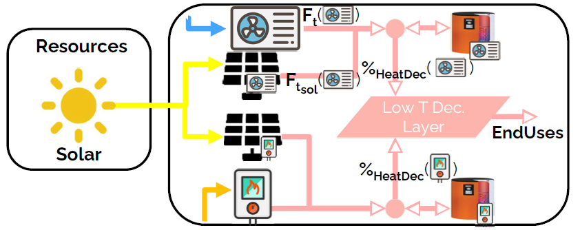
Fig. 11 Illustrative example of a decentralised heating layer with thermal storage, solar thermal and two conventional production technologies, gas boilers and electrical HP. In this case, Eq. (29) applied to the electrical HPs becomes the equality between the two following terms: left term is the heat produced by: the eHPs (\(\textbf{F}_{\textbf{t}}('eHPs',h,td)\)), the solar panel associated to the eHPs (\(\textbf{F}_{\textbf{t}_\textbf{sol}}('eHPs',h,td)\)) and the storage associated to the eHPs; right term is the product between the share of decentralised heat supplied by eHPs (\(\textbf{%}_{\textbf{HeatDec}}('eHPs')\)) and heat low temperature decentralised demand (\(\textbf{EndUses}(HeatLowT,h,td)\)).

A thermal storage \(i\) is defined for each decentralised heating technology \(j\), to which it is related via the set TS OF DEC TECH, i.e. \(i\)=TS OF DEC TECH(j). Each thermal storage \(i\) can store heat from its technology \(j\) and the associated thermal solar \(\textbf{F}_{\textbf{sol}}\) (\(j\)). Similarly to the passenger mobility, Eq. (29) makes the model more realistic by defining the operating strategy for decentralized heating. In fact, in the model we represent decentralized heat in an aggregated form; however, in a real case, residential heat cannot be aggregated. A house heated by a decentralised gas boiler and solar thermal panels should not be able to be heated by the electrical heat pump and thermal storage of the neighbours, and vice-versa. Hence, Eq. (29) imposes that the use of each technology (\(\textbf{F}_{\textbf{t}}(j,h,td)\)), plus its associated thermal solar (\(\textbf{F}_{\textbf{t}_\textbf{sol}}(j,h,td)\)) plus its associated storage outputs (\(\textbf{Sto}_{\textbf{out}}(i,l,h,td)\)) minus its associated storage inputs (\(\textbf{Sto}_{\textbf{in}}(i,l,h,td)\)) should be a constant share (\(\textbf{%}_{\textbf{HeatDec}}(j)\)) of the decentralised heat demand \((\textbf{EndUses}(HeatLowT,h,td)\)). Figure 11 shows, through an example with two technologies (a gas boiler and a HP), how decentralised thermal storage and thermal solar are implemented.

Vehicle-to-grid

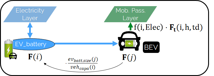
Fig. 12 Illustrative example of a V2G implementation. The battery can interact with the electricity layer. The size of the battery is directly related to the number of cars (see Eq. (30)). The V2G takes the electricity from the battery to provide a constant share (\(\textbf{%}_{\textbf{PassMob}}\)) of the passenger mobility layer (Mob. Pass.). Thus, it imposes the amount of electricity that electric car must deserve (see Eq. (31)). The remaining capacity of battery available can be used to provide V2G services (see (32)).

(30)\[\textbf{F} (i) = \frac{\textbf{F} (j)}{ veh_{capa} (j)} ev_{batt,size} (j) ~~~~~~ \forall j \in V2G, i \in \text{EVs_BATT OF V2G}(j)\]

Vehicle-to-grid dynamics are included in the model via the V2G set. For each vehicle \(j \in V2G\), a battery \(i\) (\(i\) \(\in\) EVs_BATT) is associated using the set EVs_BATT_OF_V2G (\(i \in \text{EVs_BATT_OF_V2G}(j)\)). Each type \(j\) of V2G has a different size of battery per car (\(ev_{batt,size}(j)\)), e.g. the first generation battery of the Nissan Leaf (ZE0) has a capacity of 24 kWh [10]. The number of vehicles of a given technology is calculated with the installed capacity (F) in [km-pass/h] and its capacity per vehicles (\(veh_{capa}\) in [km-pass/h/veh.]). Thus, the energy that can be stored in batteries F(\(i\)) of V2G(\(j\)) is the ratio of the installed capacity of vehicle by its specific capacity per vehicles times the size of battery per car (\(ev_{batt,size}(j)\)), Eq. (30). As an example, if this technology of cars covers 10 Mpass-km/h, and the capacity per vehicle is 50.4 pass-km/car/h (which represents an average speed of 40km/h and occupancy of 1.26 passenger per car); thus, the amount of BEV cars are 0.198 million cars. And if a BEV has a 24kWh of battery, such as the Nissan Leaf (ZE0), thus, the equivalent battery has a capacity of 4.76 GWh.

(31)\[ \begin{align}\begin{aligned}\textbf{Sto}_\textbf{out} (j,Elec,h,td) \geq - f(i,Elec) \textbf{F}_\textbf{t} (i,h,td)\\\forall i \in V2G , \forall j \in \text{EVs_BATT OF V2G}(j), \forall h \in H, td \in TD\end{aligned}\end{align} \]

Eq. (31) forces batteries of electric vehicles to supply, at least, the energy required by each associated electric vehicle technology. This lower bound is not an equality; in fact, according to the V2G concept, batteries can also be used to support the grid. Figure 12 shows through an example with only BEVs how Eq. (31) simplifies the implementation of V2G. In this illustration, a battery technology is associated to a BEV. The battery can either supply the BEV needs or sends electricity back to the grid.

(32)\[ \begin{align}\begin{aligned}\textbf{Sto}_\textbf{in} (j,l,h,td)t_{sto_{in}}(\text{j}) + \Big(\textbf{Sto}_\textbf{out}(j,l,h,td) + f(i,Elec) \textbf{F}_\textbf{t} (i,h,td) \Big) \cdot t_{sto_{out}}(\text{j})\\\leq \Big( \textbf{F} (j) - \frac{\textbf{F} (j)}{ veh_{capa} (j)} ev_{batt,size} (j) \Big) \cdot \%_{sto_{avail}}(j)\\\forall i \in V2G , \forall j \in \text{EVs_BATT OF V2G}(j) , \forall l \in L, \forall h \in H, \forall td \in TD\end{aligned}\end{align} \]

Eq. (32) limits the availability of batteries to the number of vehicle connected to the grid. This equation is similar to the one for other type of storage (see Eq. (19)); except that a part of the batteries are not accounted, i.e. the one running (see Eq. (31)). Therefore, the available output is corrected by removing the electricity powering the running car (here, \(f(i,Elec) \leq 0\)) and the available batteries is corrected by removing the numbers of electric cars running (\(\frac{\textbf{F} (j)}{ veh_{capa} (j)} ev_{batt,size} (j)\)).

(33)\[ \begin{align}\begin{aligned}\textbf{Sto}_\textbf{level} (j,t) \geq \textbf{F}[i] soc_{ev}(i,h)\\\forall i \in V2G , \forall j \in \text{EVs_BATT OF V2G}(j) , \forall t \in T| \{h,td\} \in T\_H\_TD\end{aligned}\end{align} \]

For each electric vehicle (\(ev\)), a minimum state of charge is imposed for each hour of the day big(\(soc_{ev}(i,h)\)big). As an example, we can impose that the state of charge of EV is 60% in the morning, to ensure that cars can be used to go for work. Eq. (33) imposes, for each type of V2G, that the level of charge of the EV batteries is greater than the minimum state of charge times the storage capacity.

Peak demand

(34)\[ \begin{align}\begin{aligned}\textbf{F} (j) \geq \%_{Peak_{sh}}\max_{h\in H,td\in TD}\left\{\textbf{F}_\textbf{t}(j,h,td)\right\}\\\forall j \in \text{TECH OF EUT} (HeatLowTDEC) \setminus \{ 'Dec_{Solar}'\}\end{aligned}\end{align} \]

(35)\[ \begin{align}\begin{aligned}\sum_{\hspace{3cm}j \in \text{TECH OF EUT} (HeatLowTDHN), i \in \text{STO OF EUT}(HeatLowTDHN)}\\\Big( \textbf{F} (j)+ \textbf{F} (i)/t_{sto_{out}}(i,HeatLowTDHN) \Big)\\\geq \%_{Peak_{sh}} \max_{h\in H,td\in TD} \big\{ \textbf{EndUses}(HeatLowTDHN,h,td) \big\}\end{aligned}\end{align} \]

Finally, Eqs. (34) - (35) constrain the installed capacity of low temperature heat supply. Based on the selected TDs, the ratio between the yearly peak demand and the TDs peak demand is defined for space heating (\(\%_{Peak_{sh}}\)). Eq. (34) imposes that the installed capacity for decentralised technologies covers the real peak over the year. Similarly, Eq. (35) forces the centralised heating system to have a supply capacity (production plus storage) higher than the peak demand. These equations force the installed capacity to meet the peak heating demand, i.e. which represents, somehow, the network adequacy [11].

Adaptations for the case study

Additional constraints are required to implement scenarios. Scenarios require six additional constraints (Eqs. (36) - (42)) to impose a limit on the GWP emissions, the minimum share of RE primary energy, the relative shares of technologies, such as gasoline cars in the private mobility, the cost of energy efficiency measures, the electricity import power capacity and the available surface area for solar technologies.

(36)\[\textbf{GWP}_\textbf{tot} \leq gwp_{limit}\]

(37)\[ \begin{align}\begin{aligned}\sum_{j \in \text{RES}_\text{re},t \in T| \{h,td\} \in T\_H\_TD(t)} \textbf{F}_\textbf{t}(j,h,td) \cdot t_{op} (h,td)\\\geq re_{share} \sum_{j \in \text{RES} ,t \in T| \{h,td\} \in T\_H\_TD(t)} \textbf{F}_\textbf{t}(j,h,td) \cdot t_{op} (h,td)\end{aligned}\end{align} \]

To force the Belgian energy system to decrease its emissions, two lever can constraint the annual emissions: Eq. (36) imposes a maximum yearly emissions threshold on the GWP (\(gwp_{limit}\)); and Eq. (37) fixes the minimum renewable primary energy share.

(38)\[ \begin{align}\begin{aligned}f_{\text{min,\%}}(j) \sum_{j' \in \text{TECH OF EUT} (eut),t \in T|\{h,td\} \in T\_H\_TD(t)} \textbf{F}_\textbf{t}(j',h,td)\cdot t_{op}(h,td)\\\leq \sum_{t \in T|\{h,td\} \in T\_H\_TD(t)} \textbf{F}_\textbf{t} (j,h,td)\cdot t_{op}(h,td)\\\leq f_{\text{max,\%}}(j) \sum_{j'' \in \text{TECH OF EUT} (eut),t \in T|\{h,td\} \in T\_H\_TD(t)} \textbf{F}_\textbf{t}(j'',h,td)\cdot t_{op}(h,td)\\\forall eut \in EUT, \forall j \in \text{TECH OF EUT} (eut)\end{aligned}\end{align} \]

To represent the Belgian energy system in 2015, Eq. (38) imposes the relative share of a technology in its sector. Eq. (38) is complementary to Eq. (9), as it expresses the minimum (\(f_{min,\%}\)) and maximum (\(f_{max,\%}\)) yearly output shares of each technology for each type of EUD. In fact, for a given technology, assigning a relative share (e.g. boilers providing at least a given percentage of the total heat demand) is more intuitive and close to the energy planning practice than limiting its installed size. \(f_{min,\%}\) and \(f_{max,\%}\) are fixed to 0 and 1, respectively, unless otherwise indicated.

(39)\[\textbf{F}(Efficiency) = \frac{1}{1+i_{rate}}\]

To account for efficiency measures from today to the target year, Eq. (39) imposes their cost. The EUD is based on a scenario detailed in Data for end use demand and has a lower energy demand than the “business as usual” scenario, which has the highest energy demand. Hence, the energy efficiency cost accounts for all the investment required to decrease the demand from the “business as usual” scenario and the implemented one. As the reduced demand is imposed over the year, the required investments must be completed before this year. Therefore, the annualisation cost has to be deducted from one year. This mathematically implies to define the capacity of efficiency measures deployed to \(1/ (1+i_{rate})\) rather than 1. The investment is already expressed in €₂₀₁₅.

(40)\[\textbf{F}_{\textbf{t}}(Electricity,h,td) \leq elec_{import,max} ~~~~~~ \forall h \in H, \forall td \in TD\]

(41)\[\textbf{F}_{\textbf{t}}(i,h,td) \cdot t_{op} (h,td) = \textbf{Import}_{\textbf{constant}}(i) ~~~~~~ \forall i \in \text{RES_IMPORT_CONSTANT}, h \in H, \forall td \in TD\]

Eq. (40) limits the power grid import capacity from neighbouring countries based on a net transfer capacity (\(elec_{import,max}\)). Eq. (41) imposes that some resources are imported at a constant power. As an example, gas and hydrogen are supposed imported at a constant flow during the year. In addition to offering a more realistic representation, this implementation makes it possible to visualise the level of storage within the region (i.e. gas, petrol …).

Caution

Adding too many ressource to Eq. (41) increase drastically the computational time. In this implementation, only resources expensive to store have been accounted: hydrogen and gas. Other resources, such as diesel or ammonia, can be stored at a cheap price with small losses. By limiting to two types of resources (hydrogen and gas), the computation time is below a minute. By adding all resources, the computation time is above 6 minutes.

(42)\[ \begin{align}\begin{aligned}\textbf{F}(PV)/power\_density_{pv}\\+ \big( \textbf{F}(Dec_{Solar}) + \textbf{F}(DHN_{Solar}) \big)/power\_density_{solar~thermal} \leq solar_{area}\end{aligned}\end{align} \]

In this model version, the upper limit for solar based technologies is calculated based on the available land area (solararea) and power densities of both PV (\(power\_density_{pv}\)) and solar thermal (\(power\_density_{solar~thermal}\)), Eq. (42). The equivalence between an install capacity (in watt peaks Wp) and the land use (in \(km^2\)) is calculated based on the power peak density (in [Wp/m\(^2\)]). In other words, it represents the peak power of a one square meter of solar panel. We evaluate that PV and solar thermal have a power peak density of \(power\_density_{pv}\) =0.2367 and \(power\_density_{solar~thermal}\) =0.2857 [GW/km\(^2\)] [12]. Thus, the land use of PV is the installed power (\(\textbf{F}(PV)\) in [GW]) divided by the power peak density (in [GW/km\(^2\)]). This area is a lower bound of the real installation used. Indeed, here, the calculated area correspond to the installed PV. However, in utility plants, panels are oriented perpendicular to the sunlight. As a consequence, a space is required to avoid shadow between rows of panels. In the literature, the ground cover ratio is defined as the total spatial requirements of large scale solar PV relative to the area of the solar panels. This ratio is estimated around five ³⁰, which means that for each square meter of PV panel installed, four additional square meters are needed.

Implementation

The formulation of the MILP and LP problems has been implemented using an algebraic modeling language. The latter allows the representation of large LP and MILP problems. Its syntax is similar to AMPL, which is - according to the NEOS-statistics [13] - the most popular format for representing mathematical programming problems. The formulation enable the use of different solvers as open sources ones, such as GLPK, or commercial ones, such as CPLEX or Gurobi. In the code, each of the equations defined above is found as it is with the corresponding numbering. SETS, Variables and parameters have the same names (unless explicitly stated in the definition of the term). Figure 13 illustrates - for the balance constraint (13) - the mathematical formulation presented in this work and its implementation in the code. Colors highlight the same elements. In the implementation, each constraint has a comment (starting with #) and has a name (colored in black), in this case layer_balance. In addition, most of the SETS, Variables and parameters are more explicitly named, as a first example the set layers is named L in the paper and LAYERS in the implementation; or as another example, the input efficiency who is named f in the paper and layers_in_out in the implementation.

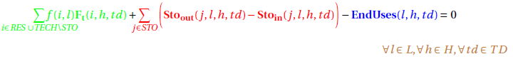
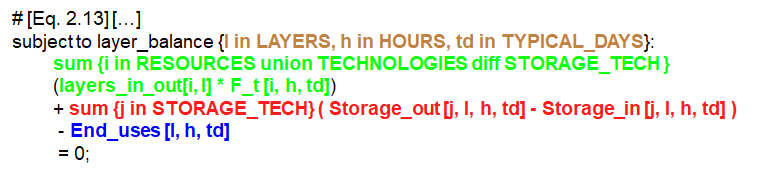
Fig. 13 Comparison of equation formulation (upper equation) and code implementation (lower figure). Example based on Eq. (13).

The entire implementation is available on the directory ³¹ and its architecture is illustrated in Figure 14. Four folders compose the repository and contain the documentation (Documentation), the data used (Data_management), the MILP implementation (STEP_1_TD_selection) and the LP implementation (STEP_2_Energy_Model). For each of the models, the definition of the terms (SETS, Variables and Parameters) as well as the domains of the variables, the formulation of the constraints and the objective function are included in the model file (with the extension .mod). The numerical values of the parameters are contained in separate files (with the extension .dat). Finally, the output data of the model are saved in a file (wit the extension .out) or a folder (\outputs). An interface - via excel - allows to visualise the data (DATA.xlsx) and to generate the data files (STEP_1_in.xlsx, STEP_1_out.xlsx and STEP_2_in.xlsx). Finally, a user guide manual is available in the documentation to support the modeler in her/his first steps.

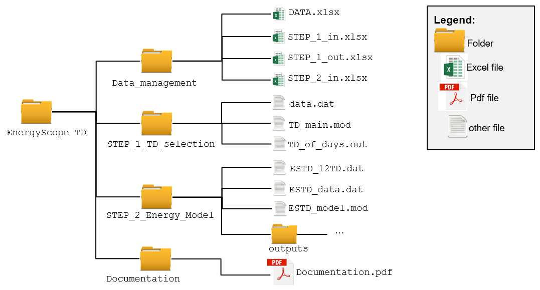
Fig. 14 EnergyScope TD repository structure available at ³¹.

[1]

Passenger transport activity from aviation is accounted in passenger mobility (excluding international extra EU travels).

[2]

Hydrogen can be produced based on many feed-stocks, among them electricity used for electrolysers.

[3]

Indeed, some technologies have several outputs, such as a CHP. Thus, the installed size must be defined with respect to one of these outputs. As an example, CHP are defined based on the thermal output rather than the electrical one.

[4]

To simplify the reading, the formulation \(t \in T| \{h,td\} \in T\_H\_TD(t)\) is used. However, this cannot be directly implemented in the code and it requires two additional sets : \(HOUR\_OF\_PERIOD(t)\) and \(TYPICAL\_DAY\_OF\_PERIOD(t)\). Hence, we have: \(t \in T| \{h,td\} \in T\_H\_TD(t)\), which is equivalent in the code to \(t \in T| h \in HOUR\_OF\_PERIOD(t), td \in TYPICAL\_DAY\_OF\_PERIOD(t)\).

[5]

In most cases, the activation of the constraint stated in Eq. (14) will have as a consequence that the level of storage be the same at the beginning and at the end of each day — hence the use of the terminology ‘daily storage’. Note, however, that such daily storage behaviour is not always guaranteed by this constraint and thus, depending on the typical days sequence, a daily storage behaviour might need to be explicitly enforced.

[6]

In the code, these equations are implemented with a if-then statement.

[7]

In this linear formulation, storage technologies can charge and discharge at the same time. On the one hand, this avoids the need of integer variables; on the other hand, it has no physical meaning. However, in a cost minimization problem, the cheapest solution identified by the solver will always choose to either charge or discharge at any given \(t\), as long as cost and efficiencies are defined. Hence, we recommend to always verify numerically the fact that only storage inputs or outputs are activated at each \(t\), as we do in all our implementations.

[8]

This is the ratio between the losses in the grid and the total annual electricity production in Belgium in 2015 ³².

[9]

[foot:nonLinear]All equations expressed in a compact non-linear form in this section Eqs. (24), (25), (29) and (35) can be linearised. For these cases, the EndUses is defined with parameters and a variable representing a constant share over the year (e.g. \(\textbf{%}_\textbf{public}\)). As an example, EndUses in Eq. (24) is equal to \(\textbf{EndUsesInput}(PassMb) \cdot %pass (h, td) / t_op (h, td)\). The term \(\textbf{%}_{\textbf{public}}\), is missing in the equation, but is implicitly implemented in \(\textbf{%}_{\textbf{PassMob}}\).

[10]

This generation (ZE0) was marketed from 2010 to 2017 with a battery capacity of 24 kWh. The new generation (ZE1) accounts for an improved capacity and reaches 40 kWh per battery. Data from https://en.wikipedia.org/wiki/Nissan_Leaf, consulted on 08-02-2021

[11]

The model resolution of the dispatch is not accurate enough to verify the adequacy. As one model cannot address all the issues, another approach has been preferred: couple the model to a dispatch one, and iterate between them. Percy and Coates ³³ demonstrated the feasibility of coupling a design model (ESTD) with a dispatch one (Dispa-SET ³⁴). Based on a feedback loop, they iterated on the design to verify the power grid adequacy and the strategic reserves. Results show that the backup capacities and storage needed to be slightly increased compared to the results of the design model alone.

[12]

The calculation is based on the annual capacity factor, the conversion efficiency and the average yearly irradiation. As an example, for PV, the efficiency in 2035 is estimated at 23% ³⁵ with an average daily irradiation - similar to historical values - of 2820 Wh/m\(^2\) in Belgium ³⁶. The capacity factor of solar is around 11.4%, hence specific area for 1 kilowatt peak (\(kW_p\)) is \(2820/24\cdot0.23/0.114\approx236.7\)[\(MW_p\)/km\(^2\)]=\(0.2367\) [\(GW_p\)/km\(^2\)].

[13]

NEOS Server is an Internet-based client-server application that provides free access to a library of optimization solvers, statistics are available at: https://neos-server.org/neos/report.html, consulted the 27/01/2021.